Here you'll find a list of common Microsoft Excel formulas and functions explained in plain English, and applied to real life examples.
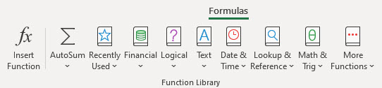
The tutorials are grouped in line with the Function Library so they're easy to find when you need them.
And when you're ready to take your skills to the next level check out our Excel training course.
The Basics
Absolute References Explained - These are the $ signs you see in formulas, and they should be one of the first things you learn.
Formulas Not Working? Get help here. In this video I share several tips that will help you understand any formula and why it's not returning the correct result.
Tabular Data - the perfect data format and 5 other formats that will make your life difficult.
Writing Formulas Efficiently - In this post I share how to write formulas in such as way that it’s quick to write, and quick to maintain.
Named Ranges - have so many applications and are a great time saving tip that makes building and deciphering formulas much quicker and easier
Date and Time calculations - If you haven't done so already it won't be long before you have to work with time and dates. Here are some fundamental rules.
Space Operator - is not very well known, but you can put it to a range of uses. Pull this trick out at parties and people will think you're some kind of superhero 😉
Dynamic Arrays - new for Office 365 users and while not basic, Dynamic Arrays fundamentally change the Excel calc engine, therefore Excel users of all levels should at least be aware of them.
Logical Functions
IF Function - enables you to perform logical tests on your data. You can then tell Excel what to do if the test evaluates to TRUE, or if it evaluates to FALSE.
IFERROR – New in Excel 2007, this function allows you to hide the errors returned by formulas. A great example is when VLOOKUP evaluates to #N/A. No more nested IF(ISNA... formulas slowing down your workbook. Plus IFERROR is much more efficient and easy to understand.
Nested IF Formulas – This extends the number of criteria you can test but don’t get carried away nesting too many IF’s though.
IF, OR and AND used together – Now we’re cooking with fire. Nesting OR and AND with IF gives you even more logic to play with, extending the functionality of IF.
Lookup & Reference
VLOOKUP Exact Match version – This is my all-time favourite. Not because it’s the best, but because it’s one of the first I learnt that unleased the power of Excel for me. Check out the video tutorial as well as written lesson.
VLOOKUP Sorted List version – I discovered this version of VLOOKUP a long time after I’d master the exact match method. Although very similar, this allows you to apply it in quite a different way.
VLOOKUP with dynamic column reference – Enables you to automate updating the col_index_num argument so you can copy VLOOKUP across columns and not need to edit it.
VLOOKUP and Sum Multiple Columns – this allows you to lookup a value and sum a group of columns.
VLOOKUP Multiple Criteria - enables you to specify multiple criteria in your lookup value.
VLOOKUP Multiple Sheets – 3D VLOOKUP which enables you to look up many worksheets to locate the lookup value.
VLOOKUP Multiple Values in Multiple Columns – enables you to lookup multiple values and match them to multiple columns before returning your result. It uses a quirky IF function trick. I also show you how to do the same thing with INDEX & MATCH.
VLOOKUP with CHOOSE - a trick that allows you to look up columns to the left.
Lookup and Return Multiple Values – enables you to find multiple matches and return multiple results
HLOOKUP Exact Match and Sorted List - these are the same as VLOOKUP's except on rows of data instead of columns.
INDEX and MATCH - a VLOOKUP alternative that solves some of its limitations like looking up to the left.
CHOOSE - on its own it isn't all that special, but when you team it up with some other functions they become very clever.
OFFSET - a lot of people struggle to understand how the OFFSET function works, but I make it easy with my treasure map analogy.
OFFSET - Dynamic Reference Video
INDIRECT Function - this is best known for fixing a range of cells you want to reference.
HYPERLINK Function - hyperlinks can be inserted using the hyperlink tool, or you can write a formula. Here I share with you a shortcut to inserting hyperlink formulas.
ROW, ROWS, COLUMN and COLUMNS functions - you've probably seen these functions nested in formulas and wondered what they're doing there. All is revealed in this tutorial.
Financial Functions
Excel Bank Reconciliation Formula - how to match debits and credits in a spreadsheet.
FV - for calculating compound interest on Savings
NPER - calculate how long it'll take you to become a millionaire 🙂
ACCRINT - calculates the accrued interest for a security that pays interest periodically.
Math & Trig
SUMIF & SUMIFS Explained - SUMIF enables you to employ logic to what you sum, and if you have Excel 2007 or later you can use the SUMIFS function to sum data based on multiple criteria.
SUBTOTAL Explained - this is one of those best kept secrets. It has so many different applications it's a wonder more people don't know about it.
ROUND, ROUNDUP, ROUNDDOWN - rounding numbers is made easy with this trio.
FLOOR and CEILING - These enable you to round the decimal places of a value to be divisible by a number you specify. For example, rounding up or down to the nearest 5 cents.
RAND and RANDBETWEEN - I use these all the time to generate random data for writing my tutorials but they have some other clever uses too.
SUMPRODUCT - is not only a great alternative for Excel 2003 users who wish they had SUMIFS, AVERAGEIFS and COUNTIFS. But it also has some other advantages which makes it more flexible than the *IFS range of built in functions.
Statistical Functions
AVERAGE, AVERAGEIF and AVERAGEIFS - these are much like SUM, SUMIF and SUMIFS except for average. No surprises there! But I also show you a clever way to use AVERAGEIFS with a data validation list to make it dynamically update.
COUNT, COUNTA and COUNTBLANK Functions - counting in Excel can be a bit tricky depending on whether you want to count numbers or text or both. Here I show you the ropes.
COUNTIF & COUNTIFS Explained - If you've used SUMIF/IFS you can probably guess that these functions allow you to count based on criteria. Here I show you a few examples using COUNTIF and COUNTIFS plus a video tutorial.
STDEV & STDEVP Explained - I remember Standard Deviation from my accounting days. Thankfully you can put away the calculator because it can be easily done in Excel.
MIN, MAX, SMALL and LARGE - there's more to these that meets the eye. Here I share a couple of clever ways to use them.
RANK, RANK.AVG and RANK.EQ - We all want to know who came 1st, 2nd, 3rd, but what if there's a tie? Check out this post to see solutions to tie breaks and other clever uses.
Between Formula using MEDIAN - there's no such function as BETWEEN so here is a workaround using MEDIAN.
TRIMMEAN IF... - find the average IF criteria is met, and excludes outliers.
Text Functions
ISTEXT, ISNUMBER and ISBLANK. - Logical tests you can use to test if a range contains text, numbers or is empty.
TEXT - enables you to convert numbers to text. You might wonder why you'd ever need this so I've included some examples and a clever twist.
T Function - this is one of the shortest functions but it can have a big impact in the right scenario. Here I show you a few different ways you can put it to work.
UPPER, LOWER and PROPER - When you import data from another source it can often need tidying up before you can use it. These enable you to fix the case quickly and easily.
SUBSTITUTE - This is similar to find and replace except in formula form.
TRIM, CHAR and SUBSTITUTE - Use TRIM to remove spaces at the beginning and end of text. CHAR allows you to display characters by entering their code number. This is great if you want to show a character not on your keyboard. In this example I show you how you can use all 3 to handle the non-breaking space that sometimes gets imported when you copy data from a web page.
Nested SUBSTITUTE trick - Replace multiple items in one value.
CLEAN - This is great for cleaning data copied from a web page which contains some funky and usually unwanted characters.
CONCATENATE - there comes a time when you need to join text together. You can use the CONCATENATE function or you can use the ampersand symbol. I prefer the ampersand as it's much quicker to type, but here I show you both methods.
SEARCH and FIND - These two are very similar. The main difference is SEARCH is not case sensitive, whereas FIND is.
5 Step System for nesting MID functions to extract text strings.
MID, LEN, REPT and FIND - Rearranging data often requires teamwork from a myriad of functions. These are the usual suspects you'll need to tackle most text rearranging jobs.
Date and Time Functions
Excel Date and Time - Everything you need to know about working with Dates and Time in excel.
Calculating Time in Excel - How time works in Excel and number formats to add cumulative time.
Rounding time and converting time to decimals - working with time in Excel can be quite challenging if you don't know these tricks. Here I share with you my Date and Time 101, including a clever way to handle the problem of negative time often encountered when calculating hours worked by shift workers.
TIME - Here I share a workbook that converts time zones.
EOMONTH - I'd be lost without EOMONTH. I use it all the time (no pun intended) with SUMIFS/AVERAGEIFS/COUNTIFS to add up data by months.
EDATE - This is great for working out due dates or how overdue something is.
DATEDIF - you'd be forgiven for having never heard of DATEDIF. You won't find it documented anywhere in Excel because it's only available for backward compatibility. Here I show you how to use DATEDIF and a myriad of uses for it. It's a shame it's so secret.
NETWORKDAYS - if you do any sort of project planning then this is a great function to have in your tool belt. In this tutorial I team it up with TODAY and EOMONTH.
Convert dates formatted as text strings to numbers - this is handy if you import data from other systems and the dates come in as text instead of real dates.
Information
N Function - another very short function but quite handy. N enables you to put notes inside your formulas, much like a programmer would annotate their code to help them and others understand their logic. That wasn't the original purpose if N, but it's handy nonetheless.
Database Functions
DSUM, DAVERAGE, DCOUNT etc. - These are a great alternative to complex and slow array formulas.
Charts
Chart Axis Label Tricks - getting your axis labels right can make a huge difference to the readability of your charts and set your work apart from the amateurs who just use the defaults./p>
Chart Secondary Axis - It won't be long before you find the need to plot data on a secondary axis. It can be used for plotting two sets of data with vastly differing ranges of values in the one chart...although it is not my preference. I prefer to separate the data into two charts then there's no confusion over which axis is for which series.
Histogram Charts - Here I show you how to use the FREQUENCY function to compile your data into bins ready for plotting in a histogram.
In-cell Charts - If you don't have Excel 2010 or later then these are an alternative to the new Sparklines.
Gantt Charts - Got a small project you're working on? You can use this simple Gantt chart to visualise your schedule.
Gantt Chart Template using Conditional Formatting - This Gantt chart can be customised to suit your needs. It's still really only good for small-ish projects.
Pivot Tables
GetPivotData - most people hate GETPIVOTDATA when they first see it but don't be put off, it is well worth mastering.
Pivot Tables Explained - If you work with large volumes of data you must learn PivotTables. They might take a bit of practice but once you learn them it's like riding a bike. You never forget and you wonder what you thought was so hard about them.
Pivot Table Tutorial - If you prefer to learn by watching as opposed to reading you can watch my PivotTable video tutorial.
Auto-refresh Pivot Tables - If you update your PivotTable data source regularly or you have lots of PivotTables in one workbook then this is a great timesaver.
Extract sub-sets of data using a Pivot Table Report,
Reverse Pivot Table - this is genius. If your data is not in the right format for a PivotTable you might be able to rearrange it in seconds using this tip.
Add a Percentage of Total Column to a Pivot Table - This is a clever way to analyse a column of values. View this tutorial as a video or read the written instructions.
Group Data in a Pivot Table - Grouping dates is a common need when working with PivotTables, but did you know you can also group ages into bands and other data. I show you how to do both in the video tutorial, or you can read the instructions.
Compare Columns in a Pivot Table - Month on month comparison of data is a common task. You can easily set up your PivotTable to do this for you. Watch my video tutorial or follow the set by step written instructions.
Slicers - New in Excel 2010 once you start using Slicers you'll wonder how you lived without them. They'll transform your PivotTables into easy to use professional looking report.
Other Tools and Tricks
Evaluate Formula Tool - If you want to see under the Excel hood then this is your secret window. It's an essential tool for debugging and writing complex formulas.
Tables and Structured References - In Excel 2007 these had a revamp and are now a must have for your tool belt. They can make writing and maintaining formulas quick and easy by utilising the automatic dynamic ranges they have known as Structured References. Learn them and you'll never look back.
Data Validation - Drop Down Lists - who doesn't like a drop down list? They have so many uses. In this tutorial I also show you a clever way you can make your data validation list dynamic.
Custom Cell and Number Format Guide - check out this comprehensive guide to custom number formats.
Conditional Formatting - There are a load of built in conditional formats you can put to work right away without too much fuss.
Conditonal Formatting with Formulas - if the built in Conditional Formats aren't cutting it you probably need to write a custom format. I tell you, they can be confusing and frustrating if you don't know these key rules.
How to Apply Filters - filters allow you to quickly analyse your data by filtering out the stuff you don't want to see.
Advanced Filters - so much more than just filters. There's a myriad of ways you can use Advanced Filters which I cover in this tutorial.
How to insert Subtotals - this tool allows you to quickly summarise your data. It automatically adds the SUBTOTALs and groups and outlines your data. I used this a lot when working with large amounts of data that I didn't want in a PivotTable but still wanted the ability to quickly summarise it.
Dynamic Named Ranges - these are an advanced trick you must know. They allow you to write formulas so that you never have to update them when you add more data to your range.
Fix date formats using Text to Columns - if you don't like the MID, LEFT and RIGHT functions for rearranging your data then Text to Columns is a much easier option for fixing up data you've imported from another source.
Extract text strings using Text to Columns
How to Join Text Together - This is the CONCATENATE and Ampersand tutorial from the 'Text Functions' section above. I've listed it again because it's a must know tip.
How to insert Outlines - Ever wondered how to insert those nice grouping buttons the Subtotal tool does for you automatically? I show you how here.
Camera Tool - It's not easy to find, but I show you where it's hiding and a great way you can use it in dashboard type reports. I also show you a cool trick where you can use it with a formula to dynamically update the picture displayed.
Shapes and SmartArt - add depth to your workbooks with Shapes and SmartArt. You can even make the text it displays dynamic. Or link them to Macros and use them as buttons plus much more.
Importing data - In this tutorial I show you how to import data from Access, Web pages and Text or CSV files. Plus how to handle importing data without delimiters.
Array Formulas - These are the formulas that have the {curly braces}. They have a few nuances which set them apart but in this tutorial I lift the lid on them and step you through the logic of how they work.
Wildcards - There are a few different types of wildcards and in this tutorial I show you how you can use them with COUNTIF, SUMIF and VLOOKUP.
Excel Workspace - this is a great time saving tip for those of us who open the same group of workbooks regularly as it allows you to list a group of workbooks together and open them with one click, plus some other cool features.
Go To Special - I love this tool. It has so many features and in this tutorial I show you how you can use it to quickly remove blanks from your data.
EVALUATE - this is another secret function you won't find in the function list. It's acutally an Excel v4.0 macro function and in this tutorial you can learn a clever way to use it with data validation lists.
Didn't find what you were looking for?
Try our blog or use the Search box at the top of the page.
Failing that you could try Microsoft themselves.
Found This Useful?
If you found our explanations useful, please help us out by sharing this page through Facebook, Twitter, and Linked In.


Good day,
I need to have the close value of he NASDAQ Composite Index (NYSE) value on my spreadsheet for a specific date. Say the 8th of June 2021.
The Stock code for
What is the formula I have to enter for this?
There’s no formula for this, Danie. You might be able to use Power Query to connect to a web page that contains this value and bring it into Excel.
I came across something recently that I have not seen mentioned anywhere. Thought it might be of interest, though it could easily be something well-known, just not to me.
I encountered it a year ago, as I now realize, though at the time I thought it was a small enhancement MS provided as I only saw the end result, not the “happening” that must have occurred.
About a month ago though, I noticed it happen. “It” being the formula editing bar expanding due to my own action. What I saw a year ago was the apparent increase of the expanded size for it from the long, long, three line display to a five line display. Even thanked them on their user forum. Not that they read much from there.
But a month ago, I saw a flash on the screen when mishandling my mouse a little and saw the display had changed to six lines. Careful mouse movement showed a standard, (up/down) double-headed pointer appearing at the bottom edge of the editing bar, actually a noticeably lower than one would expect spot, and experimentation confirmed that it would, if engaged and dragged, enlarge or contract the expanded version of the formula editing bar as much as desired. Even to the point of taking all of the screen’s real estate (so no cells display).
This has been very nice to use when writing multi-line formulas as I can see the whole thing now, not just a portion. And given how I structure LET() formulas to declare the variables in logical groupings, with the groupings separated line-wise, it’s been especially useful.
I thought I’d mention it because Jon Acampora sent an email about Alt-Enter. (Halfway through my comment about it, his website behaved bizzarely and wiped it out. For whatever reason, I often think of your site and his together, and thought you folks might be interested in it, if you didn’t, of course, already know about it.) It seems to me many of the uses of Alt-Enter might also benefit from a larger formula editing bar now and then. I know your focus is a bit past that kind of thing, usually, but you do offer a shortcut list and a couple other things that make me think you won’t be aggravated by this comment.
Thanks for sharing, Roy. I have been using this technique for so long that I probably take it for granted. I’ll keep it in mind to show in a video next time the occasion arises.
I have very big data of employees with birth dates and anniversaries, where dates and months are mentioned in separate columns.
I want formula to find and show all occurrences data of selected 2 criteria (date and month) in 2nd sheet.
Please help.
Hi Amar,
You could use PivotTables with Slicers for this report.
Mynda
Dear Mynda,
I found your website surfing on Internet and I really felt lucky about that. I’m a really fan of the excel on which I work on my day-by-day to support me in my role as manager for an italian financial company.
Thanks for your suggestions, free downloads and useful videos (which I’ve subscribed).
At the moment I’m quite interest on the excel macro (which I use through the recording mode) and the VBA functions for access.
Would you be so kind to give me some suggestion on these areas, please?
Thanks in advance for your time and feedback.
Kind regards
Daniele
Hi Daniele,
So pleased you found our training resources helpful. Here’s a list of our VBA tutorials. I hope that helps.
Mynda
Hi, I want to make a chart of my sheet1 int another sheet, Any new data I am putting in the chart1 must be added to another sheet and also to the graph.
Hi Hussy, if your chart data is stored in an Excel Table the chart will automatically pick up the new data. Alternatively, you can use dynamic named ranges to reference the data for the chart. If you get stuck please post your question and sample Excel file on our forum where we can help you further: https://www.myonlinetraininghub.com/excel-forum
I need help with a excel formula
It is a ratio question. I need to see if there is a way to do a formula where 4-16 people I need 3 supervisors and after 16 each additional 8 I need 1 leader so for example:
4-16 people requires 3 supervisors and each additional 8 people over 16 I need 1 additional supervisor.
So if I had 35 people I would need 7 supervisors or another is if I had 24 people I need 4 supervisors but if I had 25 people I would need 5 supervisors.
I hope this makes sense.
Hi Andy,
We need some more information;
1. how many supervisors do you need for 1 to 3 people?
2. Based on your examples, I think your calculation for 35 people should be 6 supervisors. Please confirm.
Please post your answers and original question on our Excel forum where you can also upload a sample file and we can help you further.
Mynda
Hi Mynda
So for 4-16 people I need 3 supervisors and for each additional 8 over the 16 I need 1 supervisor
So for 24 I need 4 supervisors or for 25 – 32 I need 5 and from 32-40 I would need 6 etc. Sorry yea I made the error there on the ratios.
Hi Andy, you haven’t answered my first question. Thanks, Mynda
Hi Mynda,
Sorry for that. The ratio is only for a min of 4 and anything under we do not allow the meeting to happen. We need a min of 4 people with 3 supervisors
4-16 = 3 supervisors
17-24=4 supervisors
25-32=5 supervisors
Hi Andy,
You can use the formula below, where A2 contains the number for the meeting:
Mynda
Hi I need help with a formula please
Hi Willem,
You can post your question on our forum.
Regards
Phil
Hi,
can you please help to separate email id using formula. for eg:- (emailto:[email protected]) if it’s written in A2, the answer in B2 should be “first_name”, the answer in C2 should be “last_name” & the answer in D2 should be “xyz.com”.
Kindly suggest,
Regards.
Hi Navin,
You need 3 formulae for this, one to extract each part of the email address
In B2
=LEFT(A2,FIND(".",A2)-1)In C2
=MID(A2,FIND(".",A2)+1,FIND("@",A2)-FIND(".",A2)-1)In D2
=RIGHT(A2,LEN(A2)-FIND("@",A2))Regards
Phil
hai
i want to change english titles in different languages called telugu and i want both at a time (english and telugu as well) can u please suggest me.
thank you
Hi Vandana,
I’m not clear on exactly what you are asking for. Can you please start a topic on the forum and attach a workbook with examples.
Regards
Phil
Hi,
I need help in creating my final result sheet, required sum of three or four column in a cell what must have decimal part 0 if original sum have decimal part between 0 and 50, 50 if equal to 51 to 90 and add 1 if greater than 90. If possible pls help me
Thnx
Kimberly
Hi Kimberly,
Please start a topic on the forum and supply your workbook with the data.
Regards
Phil
Hi Mynda
i have to create Org chart to explain the work volume in 2 different channels and show job required for new people joining the organization and sharing job description
kindly can you provide me a sample of org chart where i can learn it or work on it
your help in this matter much appreciated
Hi Sally,
Sorry, we don’t have any sample org charts we can give you, but if you get stuck please post your question in our Excel forum where we can help you out.
Kind regards,
Mynda
Using conditional formatting can I get value in color which is greater or less than my value
Example – I have values like this in other sheet…
1 = 10
2 = 20
3 = 30
4 = 40
My question is A2 have value 2 I will get result 20 so that is correct then it should be in green color if A2 is 2 if result got 30 then it should highlight red
Hi Chandu,
Please take a look here, it will help you understand how to build a formatting rule.
Cheers,
Catalin
In sr. No.s if I delete any number or write any text instead of number, all below listed numbers should be updated automatically. Which formula will be best in this case
Hi Amar,
It depends on how you want those other numbers to be updated. What result are you expecting once you delete a number or write text?
Regards
Phil
I want numbers to be updated by serial.
e.g.
Before
1
2
3
4
After Results
1
X
2
3
OR
X
1
2
3
Try the following formula in A2:
=MAX(A$1:A1)+1
Hi Catalin,
Thanks!
this formula solved my question.
🙂
Regards,
Amar
-2
I have a table which contains the employees age in range against the salary range and wanted to retrieve the number of employees with the age against the salary
Ages Salary
15-25 26-30 31-3
18-25 1 2 3
26-30 4 5 6
31-35 7 8 9
Require excel formula when the age is punch between the age and salary the corresponding value gets displayed
Example
Age 29
Sal 29
Output 5
Hi,
I’m a bit confused by the data you’ve provided. Please open a qs on the Forum and supply a workbook with your data.
Regards
Phil
regret to inform you that i could not upload any workbook for reference. Pls help with the excel formula
Salary Range
Age 15-25 26-35 36-45
18-25 1 2 4
26-30 3 5 5
31-35 4 81 1
36-40 6 8 2
Require excel formula when the age and salary is written the corresponding value with the range data of the table gets displayed in “Output”
Example
Input
Age 29
Sal 29
Output 5
Hi Sreekumar,
Please use our forum to upload a sample file with your data structure. Use our forum to sign-up, create a new topic and upload a sample file with manual examples of what you expect to see.
How do you calculate a financial – find the end result w starting amount, monthly contributions, interest pd, years or months of input being added. BUT…. the monthly amount increases each year by $10? say a 30 year period, starting input of $25/m to increase by $10/month each year? Thanks in advance
Hi Silke,
Please post this question on our Excel forum with a sample Excel file so we can help you further.
Mynda
NEW STYLE 2 YR 4 YR 6 YR 8 YR 10 YR 12 YR 14 YR 16 YR S M L XL XXL 3XL 4XL 5XL
BP-580318 BLACK 5 18 51 52 55 55 52 56 25 25 50 52 52 51 5 18
BP-580318 CHARCOAL MEL 8 20 45 47 57 51 43 52 25 51 50 23 23 45 8 20
BP-580318 GREY MEL 4 13 45 48 41 51 50 42 20 53 47 52 52 45 4 13
BP-580318 NAVY 5 15 40 42 40 53 47 51 22 14 14 23 23 40 5 15
BP-580318 OCEAN BLUE 6 9 12 14 17 14 14 12 52 55 55 52 52 12 4 15
BP-580318 RED 4 8 14 17 18 23 17 21 14 17 18 23 17 14 5 15
BP-580318 BLACK 5 1
2 YR 4 YR 6 YR 8 YR 10 YR 12 YR 14 YR 16 YR
S M L XL XXL 3XL 4XL 5XL
BP-580318 BLACK
BP-580318 CHARCOAL MEL
BP-580318 GREY MEL
BP-580318 NAVY
BP-580318 OCEAN BLUE
i need sum formula for row coloum
Hi Jayeshparmar,
Please post your question on our Excel forum and upload a sample Excel file with your data above and an example of the expected result. We’ll be able to help you further there.
Thanks,
Mynda
Hello,
I am using this formula =IF(Pivot!$A11=”Grand Total”,0,IF(Pivot!$A11=””,””,Pivot!$A11)), and it works perfect when excel is in English. I am supporting a global team and when Grand Total is in different languages the formula is not working as intended.
Is there a work around that I can use, other than hard-keying “Grand Total” in every language?
Thank you,
Petek
Hi Petek,
Maybe you could replace the reference to cell A11 with a VLOOKUP that references a table that lists all permutations of ‘Grand Total’ in the languages you support. e.g.
Mynda
Thank you, Mynda.
I will try that. Off to collecting “Grand Total” permutations around the world.
Cheers,
Hi I am no expert in excel and have spent the last couple of hours looking for the answer but to no avail. I have an excel spreadsheet and I am looking to use conditional formatting to highlight the entire row when a cell in column H contains “D” and the cell in column L does not contain the words “Payment fee.” I am struggling to find out how to write “does not contain the words “Payment fee.” in formula terms (Note the text string in column L does not just say “Payment fee.” and it is followed by differing text) I am looking to highlight all rows that have the letter D in column H but are not a payment fee. I hope that makes sense
Hi Sharon,
Can you please open a topic on our forum and supply a sample workbook with data so we can better understand what you are trying to do.
Thanks
Phil
I’m a beginner to excel and all of this looks intimidating to me, help! I really need to get set up for the entire course training. Or maybe for now just the basics so that I can use them in my new job I begin Monday 4/23/18. Looks like it will fun and exciting to learn all this knowledge!
Thanks,
Dayla
Hi Dayla,
I recommend you start with our free training course: https://www.myonlinetraininghub.com/free-registration
That will get you the basic knowledge and you can build from there.
All the best with your new job.
Mynda
sir i have a quarry .in a cell k20 the amount is 1065888. in k21 i wants amount 0- 250000 will be 0. and in k22 i wants amount 250001-500000 will be 5% of the amount. and in cell k23 i wants amount 500001-1000000 will be 20% of any value between these values and 1000001- above will be 30% of any value between these figures. kindly guide me which formula will be used.
Try this one:
=INDEX({0,0.05,0.2,0.3},MATCH(A1,{0,250001,500001,1000001},1))
CELLK20 amount is 1,200,000
Cell K21 amount will be 0% of amount 0 to 250,000
CELL K22 amount will be 5 % 0f amount 250,000 to 500,000
CELL K23 amount will be 20% of amount 500,000 to 1,000,000
CELL K 24 amount will be 30% of amount 1,000,001
SIR REFERENCE CELL IS K 20 (
I tried FORMULA GIVEN BY YOU
=INDEX({0,0.05,0.2,0.3},MATCH(A1,{0,250001,500001,1000001},1))
is not working.
Replace A1 from formula with K20 and it should work:
=INDEX({0,0.05,0.2,0.3},MATCH(K20,{0,250001,500001,1000001},1))
This will return the correct percentage. Multiply this with K20, and you will get the correct amount, in a single cell:
=K20*INDEX({0,0.05,0.2,0.3},MATCH(A1,{0,250001,500001,1000001},1))
If you want to set 4 different cells, then the formulas are quite simple:
=IF(AND(K20>=0,K20<250000),K20*0,0)
=IF(AND(K20>=250001,K20<500000),K20*0.05,0)
=IF(AND(K20>=500001,K20<1000000),K20*0.2,0)
=IF(K20>=1000001,K20*0.3,0)
TOTAL TAXABLE INCOME cell K20 1,200,000
– NCOME TAX
cell K22 upto 250,000
TAX0% NIL
250000 to 500,000 @5% 0f 2.5 lac to 500000
TAX 12500 (Cell K23 )
500,000 to 1,000,000(Cell K24) @20% 0f
100,000 (Cell K24 )
1000,001 to above (cell K25 ) @30%
60,000(Cell K25 )
8- TOTAL INCOME TAX
112500(Cell K26 )
sir this my problem how this answer will come.please guide me.
Hi Rajendra,
There is no new formulas to send you, my answer is the same. Please prepare a sample file and upload it to our forum (create a new topic after signing-up)
Make sure you prepare a manual calculated example with desired results, it will be a lot easier to understand eachother.
See you there.
dear sir i wants to use a formula for my problem. in a cell k19 the value is 160000.and i wats to use a formula in k20. the in this cell come 150000. and if the value in k19 cell is 140000 .the in cell k20 will be same i.e.140000. which formuka will be used.
L.E.:
sir in a cell k19 the value is less than 150000. i wants the same value in cell k20. if the value in k19 is more than 150000. iwants to take 150000 value in cell k20. which formula will be used. please guide me.
Hi Rajendra,
Try this formula in K20:
=IF(K19<=15000,K19,15000)
sir thanks very much for guidence. i used formula given by you.this works when the value in k19 is less than 150000. but when the value is more than 150000.this formula is putting the same value in k20. for example the value in k19 is 178000. this formula is taking 178000 in k20. iwants the maximim value in k20 is 150000.and if the value is less than 150000 in k19 .iwants the same value in k20. because it is less than 150000.
L.E.:
sorry sir mistakly i hav put sign> . your formula is correct.
Glad to hear you managed to make it work
No. of Trips (Target >8 Trips per day) Marking creteria , If No. of Trips covered>=8 & covered on time as Yes=0, else -2 Or if No. of Trips Assigned<8 & covered =assigned ontime as Yes=0, else -5
Dear Please let me how we can used this formulas in below sheet:-
No. of Trips Assigned No. of Trips Covered Is Target covered on Time Yes/No Performance marks received
Hi Sunil,
Try this:
=IF(AND(B2>=8,C2=”Yes”),0,IF(AND(A2=B2,A2<8,C2="Yes"),0,IF(AND(B2>=8,C2=”No”),-2,If(AND(A2=B2,A2<8,C2="No"),-5,"Other Cases")))), where column A is Assigned, column B=covered, column C=On Time.
Keep in mind that when Excel evaluates nested IF statements, it will stop at the fist TRUE logical test, the order of nested IF's is important.
Hi, I need to check 30 rows in a single column, if all of them are passed, if all are passed should return a sentence like “has passed the exam” or should return ” has failed in the exam”
Thanks in advance
Hi Ani,
You could use an IF formula like this:
Where the 30 rows containing the word ‘pass’ are in cells A1:A30.
Mynda
Hello Everyone – I recently adopted an ex coworker’s Job Grading Tool, and I do not understand the following 3 formulas, she created:
=IF(OR(O3=””,P3=””,Q3=””),””,VLOOKUP(VLOOKUP(P3,’Point Tables’!$M$45:$V$53,Q3/0.5),’Point Tables’!$A$4:$AN$37,O3*2,FALSE))
=IF(OR(S35),0,IF(OR(T34),0,VLOOKUP(S3,’Point Tables’!$A$43:$H$51,HLOOKUP(T3,’Point Tables’!$A$41:$H$51,2))))
=IF(OR(Y38),0,IF(OR(Z33),0,IF(OR(AA33),0,VLOOKUP(Y3,’Point Tables’!$A$73:$F$88,(HLOOKUP(Z3,’Point Tables’!$A$71:$F$88,2)))+VLOOKUP(AA3,’Point Tables’!$H$72:’Point Tables’!$I$76,2))))
Any help, translating these formulas into English would be GREATLY APPRECIATED b/c I never knew you can do a Vlookup on a Vlookup! So confused
Regards, Shawn
Hi Shawn,
These formulas could be replaced with INDEX & MATCH. Essentially they’re using a second VLOOKUP or HLOOKUP to find which column/row to return a value from. Anyhow, here are the translations:
IF O3 or P3 or Q3 are blank, then return blank, otherwise VLOOKUP the value in P3 in the Point Tables sheet range M45:M53 in the column number of range M:V that equates to Q3/.05, return an approximate match, then lookup that VLOOKUP result in the Point Tables sheet range A4:A37 and return the value from the column that equates to O3*2 in the range A4:AN37 and return an exact match.
The OR functions in the formula above are redundant. However, it reads IF S35 is TRUE then zero, if T34 is TRUE then zero, otherwise VLOOKUP the value in S3 in the Point Tables range A43:A51 and HLOOKUP the value in T3 of the Point Tables range A41:H41 and return the value from the second row (row 42) which will be the column in the range A43:H51 to return for VLOOKUP.
Again, the OR functions in this formula are redundant. It reads; IF Y38 is TRUE then zero, if Z33 is TRUE then zero, it AA33 is TRUE then zero otherwise VLOOKUP the value in Y3 in the range A73:A88 and use HLOOKUP to find which column to return by looking up the value in Z3 in the range A71:F71 and return the value from row 72, plus add the value found by VLOOKUP where it looks up the value in AA3 in the Point Tables range H72:H76 and returns the value from the second column.
I recommend you post some anonymized data in an Excel file on our forum and we can help you improve/simplify these formulas.
Mynda
Hi,
I have an excel sheet that has colum 4 colums D3, E3, F3 & G3. I want colum G3 to return the product of E3&F3 that is (G3 = E3*F3) but I want this to be applicable only when D3 has some text. Otherwise if D3 is blank, then I want G3 to return 0 or –
Colum D3 has a data validation list e.g cm, mm, m, Km etc which if not selected/empty, I want colum G to display 0 or –
Literally I only want to have an answer in G3 when all the three cells (D3, E3 & F3) have some tect/number. If any one of them is empty then G3 returns 0 or –
I hope its sounds clear for me to receive some help
Hi Changu,
You could try this:
Mynda
Hi there,
I left a msg for the helpdesk but have not heard back yet (a bit of a rush) not sure if someone checks this quicker maybe?
Is there anything in the below formula that would cause it to not work.
the first 2 are working 11.5 OZ and 20 CT the rest are not…it is pulling “other case”
=IF(AND(L8=1,M8=”11.5 OZ “),”EA”,IF(AND(L8=1,M8=”20 CT. “),”CT”, IF(AND(L8=1,M8=”22.5 GA “),”CA”, IF(AND(L8=1,M8=”24 CT “),”CT”, IF(AND(L8=1,M8=”2 LB.”),”EA”,”Other case”)))))
thanks so much!
Hi,
There is no 2.5 GA in your formula, only 22.5 GA. Note that there are 2 spaces after this entry from column M
24 CT has 3 spaces, in your formula you provided only one.
If your data is so dirty, you can use a different solution, like:
IF(AND(L7=1,ISNUMBER(SEARCH(“24 ct”,M7)))…..
this will replace the part:
IF(AND(L7=1,M7=”24 CT “)…..
Make the same change to all other nested IF’s, and it will ignore the trailing spaces, even the case. (not case sensitive).
If it should be case sensitive, use FIND instead of SEARCH, nothing else changes.
I would like to take MOS Excel 2016 exam (77-727). Would your training help me to pass the exam and if so which training should I attend?
Hi Jay,
Yes, our Excel Course available here will help you learn the skills for the exam.
Good luck with your exam.
Mynda
Hi,
I want a formula for my excel sheet. The condition is B1 has to show 100% if A1>=400 and 85% if A1 is between 300 and 400 and 70% if A1 is between 200 to 300 and 0 if A1 is less than 200.
Regards,
Rupesh
Hi Rupesh,
A better formula would be VLOOKUP with a sorted list as described here: https://www.myonlinetraininghub.com/excel-2007-%e2%80%93-vlookup-sorted-list-explained
Mynda
Please try with this formula..
=IF(E30>=400,”100%”,IF(E30>=300,”85%”,IF(E30>=200,”70%”,IF(E30<200,"0"))))
Thanks
Santhosh.K
only the formula itself will display in the cell, not the value. Any ideas or help will be greatly appreciated! Thanks ,
Curtis
Hi Curtis,
Change the format of that cell from Text to Number or General, depending on what type of values the formula will produce. (From Home Tab, Number section)
Then double click on that cell, and press enter.
Catalin
I want to calculate the conveyance and commission in excel but i am not able to make the formula of it please help me. The situation is here GM OF MARKETING DEPARTMENT WILL GET RS.3000,MANAGER OF MKT. DEPT. WILL GET RS.2000, EXECUTIVE OF MKT. DEPT. WILL GET 1000 AND OTHERS WILL GET 500 ONLY.
For Commission-In E column there is Designation like manager .executive ,gm.And in D column there is department like marketing, accounts etc.
Commission is given to marketing dept. only. Executive will get @3%,Manager @2% and GM@1% of net profit of Rs.450000.
Hi Apoorva,
Please post your question and a sample file in our Excel Forum.
Thanks,
Mynda
Good subject
please anybody help me to get details,
if I type A1 cell = Apple picture should be display in B1 cell
if I type A2 cell = orange picture should be display in B2 cell
if I type A3 cell = Grape picture should be display in B3 cell
Hi Saliha,
There are solutions without macros, like this one: Change Image
You can also try the solution from our OneDrive folder: View or Hide Images in cells
You have to change the code to make it work as you want, in this solution the image is displayed based on Mouse Over.
Catalin
its fantabulous site I have learned more formula in difference idea from this side, I have thanks to Mynda
Thanks, Mohamed! It’s great to know you’ve found our site helpful.
Mynda
This site is a fantastic resource that I use to help save time in developing training resources; thank you.
There are so many people that have a clear desire to know more about Excel to help them achieve their productivity goals. Your quick links and summary notes provide a succinct method of providing this info to others.
love it.
Hi Steven,
Thank you. it’s great to hear that we have been able to help you.
Regards
Phil
I see you doing many successful things in EXCEL and I am not smart enough to tackle the following problem using VBA. I tried for about 3 weeks and was partially successful using CMD functions but it required a lot of time editing my EXCEL file to get good info. I am using EXCEL 2010 and on Windows 8.1 operating system. In the old windows and EXCEL I could copy and paste.Not anymore…
I am trying to find a way to copy search folders and put them in an EXCEL file preferably with links to original location. I can’t find a way to create a directory listing of the files I have on various hard drive directories. If I had them in EXCEL I could sort and search for the files I want to find. I have well over 100,000 files in various directories. Any help or suggestions would be appreciated. Thanks,Darell
Hi Darrel,
Phil has written a tutorial on how to create a hyperlinked list of files in subfolders here:
https://www.myonlinetraininghub.com/create-hyperlinked-list-of-files-in-subfolders
Hope that helps.
Mynda
i have learn excel vba on my own by trial and error basis spending lot of time.first time i found a web site which gives so clear instruction to learn excel.
it is a great community service.as a buddhist i believe sharing knowledge with others make you be born with intelligence and a life time satisfaction you can get for knowing that so many others are benefitted by your kindness and knowledge.
thank you so much!
Thanks, Raja. I’m glad we could help 🙂
I’ve added Check boxes to my spreadsheet and linked it to another spreadsheet so then when checked or not it displays “True” or “False”. This isn’t appropriate for what I’m using it for so I’m trying to change this so it displays Checked = “YES” or not checked = “NO”. I can’t seem to get my IF formula to work … am I heading the right direction? Or way off base?? HELP!!
Hi Jo,
You can’t change what appears in the linked cell, but you can link another cell containing a formula to the linked cell. For example, if your linked cell is G1 then in H1 you could enter this formula:
Then in H1 you will see the Yes if the box is checked, or No if it’s not.
Hope that helps.
Mynda
Yes that does! I’ve just hidden the column with True/False and now it displays just the info that I needed! 🙂 thanks so much!!!!
Great! You’re welcom 🙂
Hi Mynda.
Always a fan.
https://www.myonlinetraininghub.com/excel-formulas is a god site for a quick view on formulas.
If i may suggest that you expand it slightly to be a little more helpful.
If you at each formula name added a few words describing what it basically is for. then you could CTRL+F the page with keywords and mind find exactly what you need.
Just a suggestiong though, since i know it is a tedious task.
Great idea, Kennet. I’ve made some updates. I hope you find it useful.
Mynda
Brilliant, Mynda.
Mynda, do you have any excel template sheets on the stock market for excel pivot table that has the ( date , high , low , close , volume , adj. close) for stock symbol information that I can use for (min. hour, day, week, month & year) of a stock web query, so i don’t have to go back to yahoo finance (historical prices). Mynda, I am 73 and have very little computer skills.
Any help you can give would be appreciated
John Pyskaty
Hi John,
Sorry, I don’t have anything like this and I’m not aware of any either. Have you tried a Google search?
Kind regards,
Mynda
Hi,
I have some “bad” data that I’m trying to purge from a spreadsheet. I have a column of e-mail addresses but many of the e-mail addresses are no good (do not have an “@” or a “.”). How can I write a formula or use a function to find all of these bad e-mail addresses in the column?
Thank you!
Hi Mike,
Let’s say your addresses are in column A starting in cell A2; you could write this formula in cell B2:
=AND(ISNUMBER(SEARCH("@",A2)),ISNUMBER(SEARCH(".",A2)))Formulas returning FALSE are ‘bad’ and you can then sort/filter to group them all together and then delete them.
Kind regards,
Mynda
Hi Mynda, thank you for the reply. I tried the formula you suggested but unfortunately it’s giving me a FALSE for every instance, not just those email addresses that do not contain an “@” or a “.”.
For example, one of the cells in the Email Address column is “www.thevest.com”. Obviously not an e-mail address, so I’d like to be able to remove that.
Another is “PHD”.
So I’m hoping to find a formula that will verify that the “@” and the “.” are missing so I can delete those instances.
Thanks again!
Hi Mike,
The formula should return a FALSE for http://www.thevest.com so it’s working correctly in that instance. Likewise for ‘PHD’. What I don’t have is an example of where the formula returns a FALSE when it should return TRUE. e.g. for [email protected] the formula should return TRUE. You can then filter to show only the FALSE results and then delete them.
It would be best if you raised a help desk ticket with your Excel file so we can see all of the data in context and you can cite examples of cells that you would expect to remove. That way we can test all of the variables.
Mynda
Mynda
Hi
I am trying to organise my “Next Action Due Column” I would like to have a field fill as red when the date contained in that field is todays date/current date. This is in order to help prioritise my to-do list. Can you advise how I would be able to do this?
Thanks
Matt
Hi Matthew,
You have to create a conditionally formatting rule for the dates range. If the dates are in column D for example (D2:D500), the formula for the conditionally formatting rule will be:
=$D6=TODAY()
To create the rule, select D2:D500, from Home tab–>Styles group-Conditional Formatting–>New Rule–>Use a formula–>Type the above formula then select your formatting.
This rule will highlight the cells that have the same date as today.
Catalin
Thanks so much. You have made my life so very easy.
Matt
You’re wellcome Matthew 🙂
which formula do i use so that i can allow users to change % rate of inflation to see its impact on costs and sell prices? let’s say the inflation rate is 10%.
thanks
Hi Esther,
Can you please upload a sample file with details of your calculations? It’s hard to understand what are you trying to do without an example.
Use our Help Desk system to upload a file.
Thanks,
Catalin
I couldn’t find what I was looking for, I don’t know what I need. I have 2 columns. One with a date and one with a number. I want to know the date and number of the most recent entry from another tab. how do I do this?
Thanks
Hi Brad,
Please use our Help Desk to upload a sample file with your calculations and details of what you are trying to achieve, it;s much easier to see your data structure to give you a functional formula, otherwise you can try a general formula to get the latest date from column C:
Cheers,
Catalin
Thanks was playing around and was able to use a Max count and Vlookup to get the correct outcome…..
You’re wellcome 🙂
kindly please tell me how i convet number into words.
Rupee 1500 in to one thousand five hundred only
Hi Ashish,
Here is a UDF posted by Phil showing how to convert numbers to words.
In the code change Dollars and cents to your local currency.
Catalin
You Are working exceptional by spreading the knowledge for Microsoft Excel. As far as me is concerned, I got Much More from your source of communication.
Thanks, Tahir. It’s great to know we are able to help you master Excel.
Mynda
I Want How To Use 2 Sheet Combined Column By Column And Match
Hi Mahesh,
You haven’t given me much to go on but I suspect this tutorial might help you:
https://www.myonlinetraininghub.com/vlookup-multiple-values-in-multiple-columns
Kind regards,
Mynda.
Hi Emman, my opinion is that operation can only be done using VBA, you can try to use this code to select the used range from a worksheet, and paste it in another worksheet:
Sub SelectUsedRange()Dim ws As Worksheet
Set ws1 = Worksheets("Sheet1")
Set ws2 = Worksheets("Sheet2")
ws1.UsedRange.AutoFilter field:=1, Criteria1:="<>"
ws1.UsedRange.Copy
ws2.Paste ws2.Range("A1")
ws1.AutoFilterMode = False
Application.CutCopyMode = False
End Sub
Cheers, Catalin
Hi Catalin,
Thanks a lot for taken time for me n given this suggestion. But i don’t think its a exact solution for the above question…actually its a interview question which i was attended last Saturday. The meaning of question is to select all non blanks (number or text or both) through macros it should be highlighted?
Hi Emman, the code will not select nonblanks, will just copy them to another sheet…
There is another way, i know it from Rick Rothstein , but it’s not so intuitive, but if you do it several times, you will see the functionality:
Here is the sequence of keys to use:
Ctrl+F
Shift+8 (basically just do a search for any value, using the asterisk “*” wildcard)
Alt+I
Ctrl+A (this will select all nonblanks actually)
Alt+F4 (to close the search window)
Cheers, Catalin
Hi! Mynda Treacy,
Thank you so much for your kindness in sharing such an informative tips and tricks to all Excel users. The formulas have been clearly explained and elaborated which can be easily understood by the readers. It really helps all of us and improve our knowledge in applying it in our job.
A very sincere gratitude to you for sharing the knowledge to all Excel users.
Thank you once again.
Sincere regards,
CL Lim
Hi CL,
Thank you for your kind words. It’s rewarding to know our tutorials are helpful.
Kind regards,
Mynda.
Thank you , this site is great and helps me a lot
Thank you
Cheers, Peter 🙂 Glad we can help.
Mynda, I hope you can help me with this. I have a worksheet containing several columns. Column A has the dates from January 1 through December 31. Column B is the name of particulars in each row. Column C is the corresponding amount in each row. I like to tell excel to give me the total amount for January in D1 and Feb in E2 and so on. Please help me with the formula and send it by email to facilitate getting my work done.
Thank you.
Hi Pete,
the formula you should use is:
You can add more criterias, if you need to.
Cheers,
Catalin
Great list of formulas, thanks for sharing 🙂
Thanks Amanda. Glad you found it useful.
hi
i am yogender andhra pradesh, India
i know knowledge in excel
i am working as excel trainer so i have learn advanced tip& tricks
your website is very use full all learners
further i would like join in online excel dashboards
please send about dashboards
thanking you
yognder
Hi Yogender,
Thanks for your kind comments. I’m glad you like our Excel Formulas list 🙂
I’ll email you direct about the Excel dashboard course.
Kind regards,
Mynda.
Hello Mynda,
Good day.
Hope you are well.
I am very interested about dashboard hope you can give me also.
I just read your message. I am just trying my luck if you can help me.
God bless to you.
Best regards,
Gamaliel.
Hi Gamaliel,
Thanks for your message. You can find out more about my Excel Dashboard course here.
Please let me know if you have any questions.
Kind regards,
Mynda.
This is an excerpt of a letter that I sent to my friends and family. “I stumbled onto this site looking for a resolution to a problem on a complicated spreadsheet I was developing. I don’t usually have an ongoing need for that kind of skill set. So retaining that information isn’t something that I would normally do unless I happen to be using it repetitively. Long story short, this site as well as My Online Training Hub has restored my faith in a simple, readable explanation of Excel formulas not to mention all of the Microsoft office software. The information is free as is 150 hrs of free training. Additionally, they offer 100 Excel tips and tricks that is nothing less than functionally superb. If you have a need for this occasional skill set, or your children or grandchildren have that need, this is the place. If you have a more pressing or ongoing need, they offer training that is remarkably inexpensive.
My problem was repetitive enough on my developing spreadsheet that I was totally stumped regardless of the research that I had done up to stumbling onto this site. I emailed them and they sent me a possible solution ( in less than 8 hours), which didn’t seem to work. They also offered to take a look at the spreadsheet if there suggestion didn’t work. I sent my template late one evening and got the answer back in less than 4 hours. Wow – in todays world??
I can’t say enough about this site and encourage you to store this email of their website in a location that you can access, should you ever have the need for this type of info. The resolution to my problem was critical if I was going to move forward with a custom made budget projection workbook. This was going to be the crux of a business that is being formed. PROBLEM SOLVED. The info is a quick and easy read.
Wow. Tanks for your kind words, Paul.
It’s rewarding to know that what we do is both appreciated and really helping people.
Warm regards,
Mynda.
Hi Sirji
can you help me formula regarding.
Hi Anil,
Sorry, I’m not sure what you mean. What formula do you need help with?
Regards
Phil