Struggling with Excel formulas can turn simple tasks into time-consuming challenges, leaving you frustrated and behind on work.
Fortunately, a treasure trove of formula productivity secrets lies hidden within Excel, waiting to be unlocked.
I'll guide you through maximizing writing formulas efficiently, turning potential struggles into streamlined success.
Table of Contents
Watch the Video

Download Excel Example File
Enter your email address below to download the sample workbook.
Inefficient References
First, let's look at a common example of an inefficient formula: below in columns A and B we have some employee data, and in columns E and F we’ve set up a COUNTIF formula (we can see the actual formula from column F in column G):
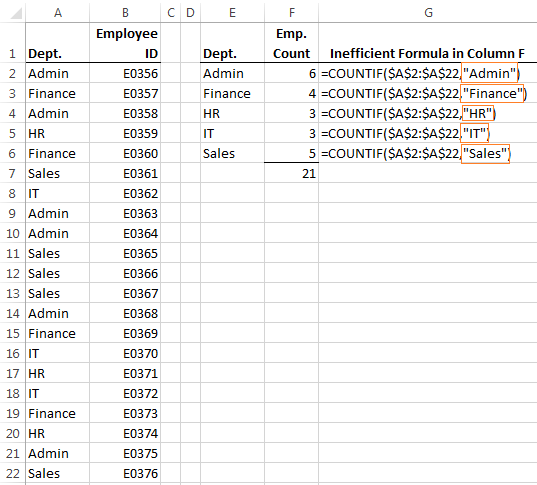
While this formula is technically correct, it's inefficient to write.
Let me explain; the ‘criteria’ argument (in the orange boxes in the image above), has been entered as text and this means each formula in column F had to be modified for each department. That's way too much work.
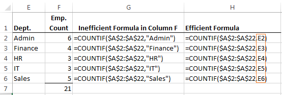
A more efficient way to write the formula is to reference a cell for the criteria argument as you can see in the example in column H below (especially since it’s right there in column E):
Formulas written this way are:
- Quick: with the efficient formula (as shown in column H above) you enter your formula in cell F2 and then copy it down the column and your job is done.
- Easy to Update: if you need to change the Dept. names in column E, your formula will automatically pick up the new name without the need to also edit the formula.
- Intuitive: where there are formulas in contiguous cells experienced Excel users will expect that the formula can be copied and pasted to all adjacent cells. So if someone inherits your file and they edit the formula, they will do so in the top left cell in the range of formulas and then copy and paste it to the remaining cells in the table. However, this could result in errors if, for example, they don't notice that your formulae 15 rows down and 3 columns to the right are subtly different because you hard keyed some criteria!
Absolute vs Relative References
Another hallmark of an efficient formula is its adept use of absolute and relative references. Those $ symbols within a formula denote whether a reference is fixed or dynamic.
Think of an absolute reference as fixing a cell's location, ensuring it remains constant, regardless of where the formula is copied to. On the other hand, a relative reference is adaptable, changing relative to the number and direction of cells it has moved.
When copying a formula, any row or column references marked by a $ symbol stay the same, signifying they're absolute. In contrast, references lacking the $ symbol automatically adjust relative to their new location.
Below is an example where absolute and relative references enable me to copy and paste one formula to many cells, earning its weight in gold; the SUMIFS formula in cell G2 (as seen in the formula bar below) can be written once and copied to the remaining 14 cells in the summary table:
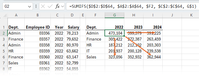
As opposed to this inefficiently written version of the formula in cell G2:
=SUMIFS($D$2:$D$64,$A$2:$A$64,"Admin",$C$2:$C$64,2022)
Notice the difference between the efficient formula and the inefficient one. The inefficient formula would require you to enter 15 different formulas, whereas the efficient formula is entered once and then copied and pasted to the remaining cells in the table.
Notice how some cell references have the column and row references absolute like this: $D$2
Some just have the column reference absolute: $F2
And others just have the row reference absolute: G$1
I won't go into detail on this here, instead you can read my tutorial on absolute and relative references.
If you haven’t mastered absolute and relative references yet I recommend you put them at the top of your ‘Excel To-Learn list’.
Named Ranges
The above tips will help you leverage Excel and absolute/relative references to do a lot of the work for you, and it's a great start but, those cell references make the formula tricky to read and write.
Let's do better by using Named Ranges instead of cell references.
For example our previous SUMIFS formula can also be written like this (see formula bar below):
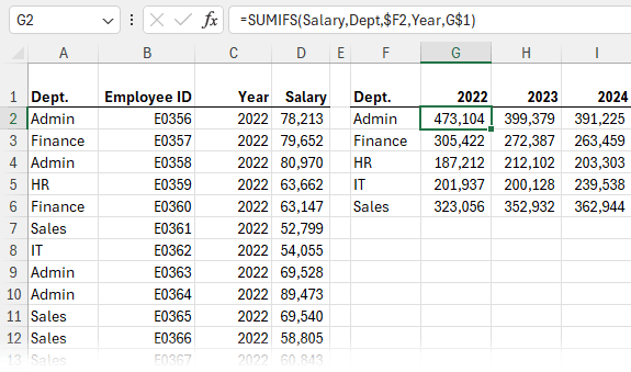
Now, isn’t that easier to read? It's also quicker to write since you can type the name of the range into the formula or press F3 to bring up the list of names to choose from.
Named ranges in their simplest form allow us to give a range of cells a name which can then be used in place of the actual cell references.
For example we can give the following ranges used in our SUMIFS formula names:
- $D$2:$D$64 name is ‘Salary’,
- $A$2:$A$64 name is ‘Dept’
- $C$2:$C$64 name is ‘Year’.
So now this formula:
=SUMIFS($D$2:$D$64,$A$2:$A$64,$F2,$C$2:$C$64,G$1)
Can be written like this:
=SUMIFS(Salary,Dept,$F2,Year,G$1)
Click here to see how to set up Named Ranges.
If you’ve mastered Named Ranges then you might be interested in Dynamic Named Ranges. These are ranges that expand and contract automatically (dynamically) as your data expands and contracts, or based on criteria you stipulate.
You can create a dynamic range using the OFFSET function or INDEX function however, if the thought of using those is a bit scary then there is a very easy way to create dynamic ranges using Excel Tables.
Excel Tables
I’m going to be blunt here; if you aren’t familiar with Excel Tables then you are missing out.
These are one of the most useful features that came out way back in Excel 2007 and yet they are one of the most underused.
The following features of Excel Tables are going to revolutionise the way you write formulas:
- Structured References: This is the name given to the way you reference cells in an Excel Table. Structured references work in a similar way to Named Ranges however, since they’re part of the Excel Table features you don’t need to set them up manually.
- Dynamic Ranges: The Structured References are dynamic; this means as you add new data to your Table the ranges automatically grow to incorporate that new data.
Structured References are a great alternative if the idea of having to get your head around complicated OFFSET or INDEX formulas to build your dynamic named ranges doesn't appeal.
Working with Structured References
There are various ways to reference the components of the Table, and in the example below you can see these particular references are made up of the table name (Table1), and column label, which we can either type in or choose from a list.
This ability to choose from a list is one of the great features of Excel Tables. As you type in part of the table/column name a list of names you can use becomes available (similar to named ranges), and you simply select the one you want.
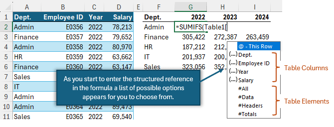
With structured references our formula in G2 becomes:
=SUMIFS(Table1[Salary],Table1[Dept.],$F2,Table1[Year],G$1)
The named ranges have been replaced with the table’s structured references (e.g. Table1[Salary] etc.)
There are many more features that come with Excel Tables which I consider a bonus:
- Filter buttons automatically applied
- Banded row formatting
- Flexible Total Row formula using Subtotal
- Automatic Freeze Pane for column labels
- Streamline your work with my Excel Tables course.
Spilled Arrays
With the introduction of Dynamic Array formulas, we can now use the hash sign shortcut to quickly reference spilled arrays.
For example, here I've used the UNIQUE Function to extract a list of the departments from column A. I can then reference the list of departments in my COUNTIF formula using the shortcut E2#. This returns a spilled array of the employee counts:
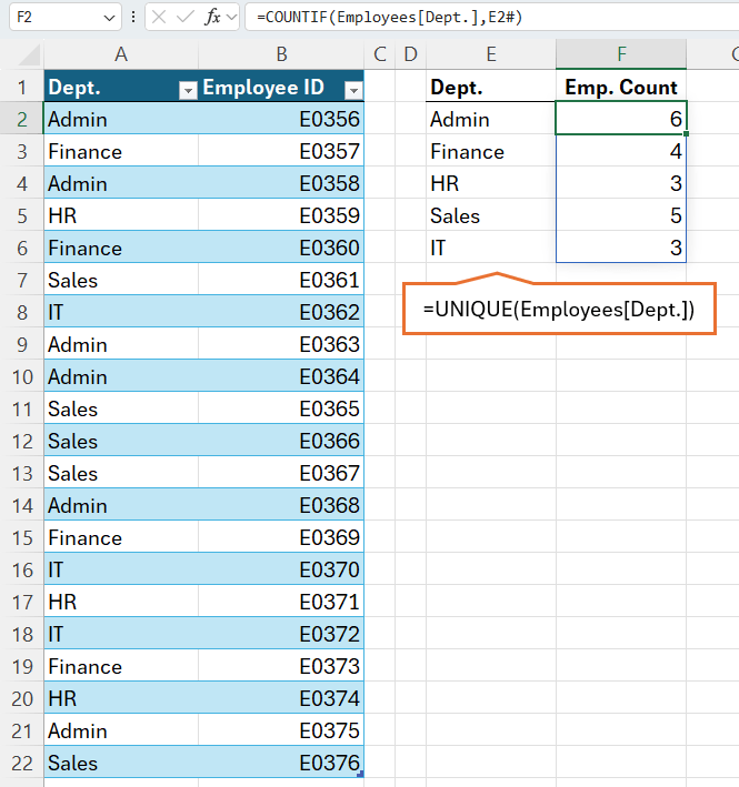
This is quicker to reference and write, plus I don't have to copy it down the column because it spills the results for me.
And if a new department gets added, the formulas automatically pick it up, as you can see in the example below for the new department, 'Operations':
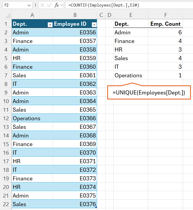
We can also reference spilled arrays in data validation lists and more. Check out this comprehensive tutorial on the spilled array operator for more tricks.
The Upshot
The bottom line is your formulas should and can be quick to write, interpret and update.
You should be aiming to write one formula for the top left cell in your table, or first cell in your column of formulas and then copy it to everywhere it needs to go. Any alterations to ranges or criteria etc. should dynamically update based on the destination of where you paste the formula.
Tools we can use to help:
- Absolute and relative references
- Named ranges
- Excel Tables
- Spilled Arrays
- Troubleshooting Excel Formulas
Next Steps
Now that you have one less Excel problem and more free time to dedicate to other important tasks. Want to save even more time? There’s a common Excel mistake most overlook, and I've explained it in this tutorial along with a solution. Check it out to avoid falling into this trap and elevate your Excel expertise even further. See you there!

There are subject codes and grades scattered in various columns & rows in excel sheet. How can I extract counted grades & codes in one cell of excel sheet, jointly.
Please workout it and sent my email address. [email protected]
for your knowledge yellow subject code 41 find out whole sheet and get answer any formula help.
CANDIDATE NAME SUBJECT CODE MRK GRD SUBJECT CODE MRK GRD SUBJECT CODE MRK GRD SUBJECT CODE MRK GRD
RAM 30 99 A1 41 95 A1 30 99 A1 41 95 A1
SHYAM 41 99 A1 48 95 A1 41 99 A1 48 95 A1
RAJ 30 94 B1 41 88 A1 30 94 B1 41 88 A1
PHILP 37 92 A2 42 80 B1 37 92 A2 42 80 B1
PIKASO 41 80 A2 42 91 A1 41 80 A2 42 91 A1
PHAS 37 93 A1 42 81 B1 37 93 A1 42 81 B1
PARI 37 90 A2 42 70 B2 37 90 A2 42 70 B2
RAJ 30 88 A2 41 68 B2 30 88 A2 41 68 B2
RAMCHARAN 41 93 A1 42 82 A2 41 93 A1 42 82 A2
ANUPAM 41 77 B1 42 82 A2 41 77 B1 42 82 A2
VIJAY 41 80 A2 42 78 B1 41 80 A2 42 78 B1
VISHAL 41 82 A2 42 73 B2 41 82 A2 42 73 B2
VINAY 37 82 B1 42 65 C1 37 82 B1 42 65 C1
VIMAL 41 72 B1 42 67 C1 41 72 B1 42 67 C1
Automatically answer will come what formula use in it.
L.E.: SUBJECT CODE 41 GET HOW MANY GRADE A1,A2,B1,B2,C1,C2,D1,D2
Hi Anil,
Please upload a sample file with your data and details on our Help Desk (create a new ticket), it will be easier to understand your situation. It will be very helpful if you create a manual result, to show us how the results should be. Also, please use Google translate to provide clear instructions in English.
Thanks for understanding.
Catalin
I have a monthly schedule I recreate in Excel every month. Is there a way to automate the dates? I have Sunday, Thursday and 2nd Saturday classes to fill in and I’m trying to get the dates to fill in based on the month.
Thanks,
Steele
Hi Steele,
I expect so but without seeing your file or a sample of your data I can’t advise as there are too many details missing. You can upload your file via the Help Desk. Please ask you question again when you raise the help desk ticket.
Thanks,
Mynda
Hi, trying to do several things with an excel file..
Im trying to group items to get the count, as well as the max date and min date for that particular subgroup.. ie for
A08 id want the result to be count = 7, min =Feb-10, Max = Jan-12
A10 id want the result to be count = 2, min = May-06, Max = Jun-10
etc…
I was trying to use the sub total function, then tried to figure out how to use the sutotal formula that gives the range of the computation (i.e. SUBTOTAL(3,C2:C8)) to then try a Min/MAX function off of the date column, but cant figure out how to get the min/max functinos to accept a cell range from a text field..
sample data.. note the full set is 6 mm + lines
Letter Code date
A08 Feb-10
A08 Feb-10
A08 Feb-10
A08 Mar-11
A08 Mar-11
A08 Jan-12
A08 Jan-12
A10 May-06
A10 Jun-10
A11 Dec-90
A11 Jun-09
A11 Apr-11
Hi Steve,
Can you please upload a sample file on our Help Desk, with details? It’s easier to work on your data structure.
Thanks for understanding.
Catalin
When calculating the hours of employees I used this formulas based on my excel data:
=a10-a11+b10-b11+c10-c11 the total hours worked
Here’s my confusion, this formula worked for 2 of the 5 employees but when using the same formula with the correct cell information it did NOT show total hours. It gave me like 01:00 or it added 10 more hours to the total…so confused and frustrated
Hi Angie,
Please upload a sample file with your calculations and details on what are you trying to do, i will gladly help you 🙂
Use our Help Hesk.
Catalin
Hi,
When using the sumifs formula with tables why is it that you cannot drag a formula in a cell across colums but you can drag it down lines. When copying the formula into columns you have to use the copy & past function.
Hi Chris,
I’m not sure why you have a problem doing this. I tested it and I can use the fill handle to drag my SUMIFS formula across the columns of a Table. Are you referring to how the structured references don’t allow you to easily assign them as absolute/relative?
Perhaps you can send me your workbook so I can see exactly what you’re trying to do. You can send it via the help desk.
Kind regarsd,
Mynda
Mynda dear
Hi
this yours work very trick nice in the excel.
thanks, kind regards
Thank you again, Manuou 🙂
i need only one formula please help
in one row student 1 got marks in diffrent subjects .there is another coloum thats is of remarks.where i want tthe formula
if student 1 got faild in 3 subjects then name of subjects ,and if fails in 4 subjects then fail must come.otherwise pass
please give me the formula
thanks and regards
hafiz muhammed ahmed
Hi Ahmed,
You can try the sample file created on our OneDrive folder.
If it’s not what you wanted, then you have to create your own data structure and upload it to our Help Desk.
Catalin Bombea
I received an Excel file of survey data spread across two sheet ( 40 rows and columns A – AE). I would like to create a report with some thing other than multiple column sorts. Any suggestions? Thanks
Hi Harry,
Without seeing the data it’s a bit difficult to suggest ways to analyse it and present it in a report. However, since you’ve collated survey data you should be trying to answer the questions that were the reason for the survey in the first place. i.e. what were you hoping to learn from the survey?
Also, sometimes it’s good to create some PivotTables from the data to help understand it and from there you might be able to identify patters/relationships.
Kind regards,
Mynda.
On “Writing Excel Formulas Efficiently”; the “SUMIFS” – I didn’t know that if you kept the “$” on just the letter ($F2) or just the number (G$1) of the formula you could copy down or copy across a specific column/row. Thanks for your fantastic site, it has helped me a lot.
Absolutely, Robin 😉
Glad we could help.
Mynda
Very good insights, especially including tables: so useful.
I would like to add one tip I always give: PPP.
Especially if you are unsure or doing something complex, start with PPP
Paper
Pencil
Plan
THAT saves a lot of time and frustration.
Duncan
I really like your Formula Tips!
One of the first things I teach people when first learning to write complex nested formulas is to create the formula one step at a time from the inside to the out side. This is especially true for formulas containing logical functions. Key is to test at each step.
The advantage is that the writer is more assured that each element of the formula is working properly. Moreover, it is easier to debug when a step is not working as expected.
Once again you provide amazing Tips and Technique to make life in the world of Excel a better place! Great tips and well described with examples so that I can easily adopt them. THANK YOU!
You are one AWESOME bundle of Excel knowledge. Thank you for this great post.
Mynda:
This is an excellent tutorial, and one to which I plan to refer my employees (and my kids, who often call asking for Excel help).
One thing you might add to your list, which I find to be a big help, is IFERROR. Occasionally a formula may legitimately result in an error; for instance, a divisor may sometimes be zero or a lookup value may not yet exist in a table. While accurate, these can spoil the looks of a report or table. =A3/B3 will result in #DIV/0! if B3 is zero, but if I use =IFERROR(A3/B3,””) instead, then I get a blank in the results rather than an error. And this is much easier than trying to do the same with just an IF statement.
In line with trying to breakproof formulae as noted in some of the comments, I have had recent issues using Excel to do lookups on data downloaded from the web. Sometimes the lookup names contain a trailing space which will invalidate the results. I have taken to using a lookup which starts assuming the value has a trailing space, and trimming it if that’s an error. This put an end to my having to rework things periodically:
=IfError(Vlookup(A1,DTable,2,FALSE),VLOOKUP(TRIM(A1,DTable,2,FALSE)
Keep up the good work!
Great tips, GJ.
Another way to use TRIM would be to put it in the VLOOKUP so every lookup value is trimmed first e.g.:
That way the VLOOKUP is only being calculated once. Not a big deal in most cases but if you’ve got a lot of VLOOKUPs you might find Excel is slow to calculate as it does the first VLOOKUP then returns and error, and then completes the second VLOOKUP. Applying TRIM to every lookup value is not a complex calculation in comparison.
Cheers,
Mynda
Hi Mynda,
Your Tips are great. As a programmer I use tables and ranges because usually table headers and ranges names are easy to understand. You should all ways remember that someone else my have to work on your formulas if you can not. Also Colin is correct you need to write so you are not all ways have to change formulas with data grows.
Great hints. This is definitely the way to go. Thanks for sharing.
all these formulas are helpful especially for me as I am using it on a daily basis with my report.. I mean most of it. I am glad that I had learned a lot from your post and helped me simplify my task..
Thanks
Eugene
@Franee, Wow! Thanks 🙂
@Eugene, Thank you. It’s rewarding to know we’re helping real people and not just sending stuff into cyberspace:-)
@Lori, It’s great to know that you find it easy to digest. when you know a topic it’s sometimes difficult to know how far in the ‘beginning’ to actually begin.
@Jef, You’re welcome.
@Milt, Glad to hear you’re one of the minority who have embraced Excel Tables.
@Skip, writing the formula inside out is a great tip. I also like to start with helper columns and then when each component is working as it should you can consolidate the formulas from the helper columns into one.
@Duncan, I like your PPP acronym. I also teach this in my Dashboard course, although I didn’t have a snappy acronym for it 🙂
Hi Mynda,
Thanks for this useful update. Just one question. When I write formulas in an xls table, as you mentioned the structured ref automatically pops-up but in that case I am confused how I should absolute them. How to insert the $ when you get Table1[Dept.] for example. Where should I put the $ sign if I want to absolute the full cell or only the column or row?
Regards,
Karine
Hi Karine,
It can be done as explained here Excel table absolute structured references
Cheers,
Mynda.
Hi Mynda,
Great post! I always say that a formula has to be like a living source, being fed continuously to stay alive. The best way to do this is to reference it to an Excel table, just like you mentioned.
As the Excel Table is fed new data in to it, the formula grows, without having to tweak it.
Static formulas tend to die off with time, unfortunately.
A good tip that I find handy for multiple function formulas is to separate them by pressing Alt+Enter, so each function has its own line in the formula bar.
Cheers, Im off to feed my formulas 🙂
Hi John,
I like the Alt+ENTER in the formula to separate nested functions. Great tip, thanks.
Hope your formulas appreciate their data dinner 😉
Mynda.
Just to add to the 3 reasons for not hard coding criteria and to expand on Col Delane’s point, my 4th point would be “Safer”.
It is too easy to forget to update the criteria or, perhaps worse, only update some of the criteria when there is a need for change. A classic over here in the UK is for VAT (sales tax) rates to be hard coded and then not updated when the rates change.
Hi Paul,
Absolutely, agree. Instead of VAT we call it GST here and the rate hasn’t changed since it was introduced. I imagine when it does change there will be a lot of ‘Find and Replace’ going on, instead of a nice quick edit to one cell.
As an alternative I also like to put criteria like that in the Name Manager like so:
Then use it in a formula e.g. calculate the GST on the value in cell A1:
Mynda.
Thanks Mynda,
I agree with most everything, especially regarding the utility of Tables. Using a formula to generate col_index_num (so that it can be copied) is also a great tip when you have a large number of contiguous vlookup references, or if the table is so extensive counting columns is error-prone. However when the number is small, or discontinuous columns are to be referenced, I find it simpler just to hard code the relevant column number.
Cheers, Gabe.
I agree, if your VLOOKUP’s don’t reference contiguous columns then hard keying the column number is the way to go.
Mynda.
I understand the issue with non-contiguous ranges, but by hard-keying the value you’re still at risk of the index No. becoming invalid through inserting or deleting columns between the lookup value and return value columns. The way I overcome this is to use the following formula to return a dynamic column index value:
=Columns([cell ref. in lookup column]:[cell ref. in return value column])
or
=Column([cell ref. in return value column]-[cell ref. in lookup column]+1)
Regards
Col Delane, Perth
Good idea to consider making it ‘break proof’. Alternatively you could use MATCH for the col_index_num.
If flexibility for your vlookup is not a critical issue and if you are talking about a very small number of columns, to hard-code the column index may not be a big problem.
But I prefer to use MATCH to identify the column index in vlookup.
Cheers,
Hi MF,
I (secretly ;-)) prefer MATCH too but if your column labels don’t ‘match’ then COLUMNS is an alternative.
Cheers,
Mynda.
Hi Mynda
Love your work – I’m often forwarding your tips to my work colleagues in an attempt to get them to understand the power of our favourite productivity tool.
Re Writing Excel Formulae Efficiently, I have a couple of comments about writing formulae that your tip clearly demonstrate:
– Here’s a question every Excel user should ask themselves every time they write a formula: “How can I write this formula so that I only need to do it once?”
– Never (well, almost never!) embed constants (e.g. “Admin” or 2012) within formulae, but rather place them in separate input cells and refer to those cells in the formula.
Regards
Col Delane, Perth
Cheers, Col.
I like your ‘question’ idea. It’s a good way to sum it up and keep it in mind.
I also agree with your theory on embedding constants. Another great place to store them is as a name in the Name Manager.
Mynda.
Hello Mynda
thank you very much for your fantastic information about Excel
it is really like a miracle information I will teach my son on this
systems once again I will Highly appreciate to your Kind help
withe my sinisterly greetings to you
Thank you, Rafi 🙂 Great to know we can help, and the more the better.
Great post! Thanks for sharing!
Thanks, Pmsocho 🙂