Excel Absolute References are the backbone of ALL formula writing enabling you to copy and paste formulas with ease.
Enter your email address below to download the sample workbook.
Excel Absolute References
You might have seen cell references in formulas surrounded by ‘$’ signs. For example $D$3:$D$10. What’s that all about?
Well, the ‘$’ before the column or row reference instructs excel to keep the reference absolute. Huh, I hear you say. Ok, I’ll explain in English.
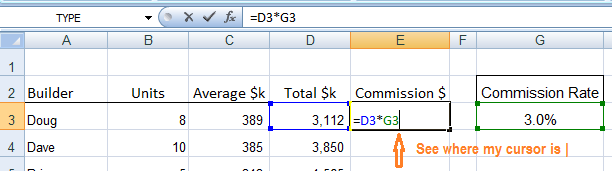
Looking at the table below we have a Commission Rate of 3% in cell G3. In column E we want to calculate the commission as Total $k x Commission Rate 3%.
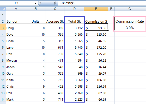
I could simply enter the formula as =D3*3% and copy it down column E, but there are two problems with this that make it not ideal:
1) I can’t easily see what the Commission Rate is without looking in the formula bar. I could put it as part of the column heading e.g. ‘Commission $ @ 3%’, but that makes my heading bigger than it needs to be, and if I change the rate at a later date I have to go back and change the heading too, which is easily overlooked.
2) If I change the rate I need to change the formula and copy it down the column again. Ok, so it might only take a few seconds to do this, but if you’re playing with scenarios and you want to change the rate a few times to see what the results are it’s much quicker and easier to just type a new figure in cell G3 and let Excel do the work to change the formula.
So assuming I’ve convinced you that referencing one cell for the commission rate is the best method let’s look at how absolute references work.
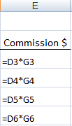
First let’s look at what happens if you don’t use an absolute reference. If you entered in cell E3 the formula =D3*G3 you would get the correct answer. But if you were to copy that formula down the rest of column E Excel would dynamically update the formula to increase by one row as it goes down the page. You can see this to the left where the reference to G3 goes G4, G5, G6 and so on.
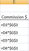
What we want Excel to do is dynamically update the cell reference to column D, but to keep the Commission Rate reference on cell G3. To do this we would use the ‘$’ signs to instruct Excel that this is an absolute reference, like this =D3*$G$3. Then when we copy the formula down the column it will be entered like example on the left here.
Other ways to use absolute references
- Make a whole range of cells an absolute reference: $D$1:$F$1
- Make only the column absolute $D3
- Make only the row absolute D$3
As you can see in the examples above, whatever the ‘$’ sign prefixes is absolute. i.e. as you copy the formula anywhere in the spreadsheet the reference prefixed by the ‘$’ sign will not change.
Shortcut to entering Absolute References
The magical F4 key instantly enters the ‘$’ signs for you. You can do it while you’re building your formula, or you can go back and edit the formula and enter them. Of course you can also type them in but it’s quicker to use F4.
Let’s look at the different ways you can enter absolute references using the F4 key in more detail
1) While you’re building your formula; as you can see below I have started to type a formula into the cell E3. I have just selected cell G3, as you can see by the marching ants (dashed line) surrounding the cell.
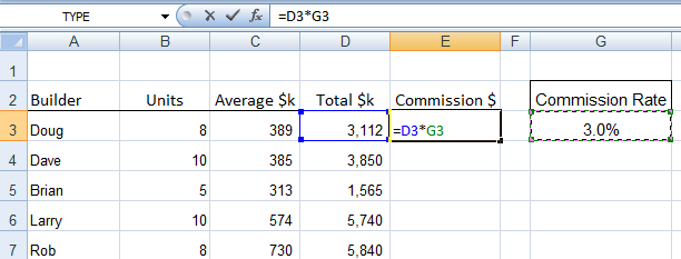
At this point, before I press enter to finish the formula, I can press the F4 key and Excel will automatically put the ‘$’ signs around G3 for me like this.

2) Or I can go back to a cell at any time and press the F2 key to edit the cell. I can then put my cursor anywhere in the cell reference I want absolute and press F4. See below.
3) If you want to absolute a range you have to highlight the cell range like the example below before pressing F4.

4) The above examples show you how to apply an absolute reference to the column and the row, but if you keep pressing F4 Excel will scroll through your options. Using =D3*G3 as an example, I want to absolute G3:
a. With the first press of F4 you will get =D3*$G$3
b. With the second press of F4 you will get =D3*G$3
c. With the third press of F4 you will get =D3*$G3
d. With the fourth press of F4 you will get =D3*G3
So, now you know how Absolute References work in Excel, and how to apply them quickly using the F4 key, you can start to build better spreadsheets that you can dynamically update.

May i know how i can make the @ in the formula? any step to use it as i try copy to new file but its not working as previous file
=IF([@IBO]>0,[@IBO]/90,IF([@PL]>0,[@PL]/180,0))
Hi,
If you intend to use the formula in a different file, you need to have the table name in front of the column reference: Table1[@IBO]
Be careful that @ refers to the current row context from that table, it does no have the same meaning if used in another file.
Thanks A lot for Such a great help, by running this Forum.
Excel was never too easy for me to understand before that.
You’re welcome.
Hi I’m having a hard time trying to write this formular. I have written it out they way I want it in the formular.
If job # equals “120” then add “Accrual Amount” to “Remaining 2017 Accrual Amount” if Job # equals “120/invoice” then subtract “invoice amount” from “Remaining 2017 Accrual Amount”
Is this something you can help with?
Can be something like this, in a new column:
=IF(A1=120,B1+C1,IF(A1=”120/invoice”,C1-D1,”Other case”))
I assume that column A has job #, Column B has Accrual Amount, column C has Remaining 2017, Column D =invoice amount, change the references to point to the real location.
You can also try our forum, you can upload there sample files if you want.
Cheers,
Catalin
Thanks Caitlin. I will try this.
Thank you for these wonderful explanations. I really enjoy your Excel tutorials. So glad I found your website.
Have an awesome day
Glad you found it helpful, Karen 🙂
very well done easy to follow thanks for the help
Glad I could help, Paul.
excellent,easy to follow thanks
Cheers, Musadiq! Glad you liked it 🙂
Excellent walk-through, easy to follow. Thank you.
Thanks, Sam!
Thanks, I will learn Excel with your help. The workbooks are great so you can instantly practice what you have just reviewed.
Glad we can help, John.
Great Explanation Mynda.
But I just curious to know that why sign $ only adopted to make freeze. why not any other sign like @.
Hi Anand,
I have no idea why the dollar sign was chosen to set absolute. I suspect it dates back to Lotus 1-2-3. Microsoft may have copied how it worked since Excel came after Lotus 1-2-3.
Mynda
Thank you so much Mynda, you are God sent.
Glad I could help, Peter.
Thoroughly enjoyed working out Absolute references 🙂 thank you
You’re welcome Kathleen.
=$E6/15-MAX(H$1:J4) help!!!!!!!!
Help with what, Jarwanna?
Hi Mynda,
I visited your website today and found it very educative and interesting. I now understand what is absolute reference. Thanks
You’re welcome Ernest, glad you found the site useful.
the following link is not working:
https://www.myonlinetraininghub.com/wp-content/moth-practice-files/Excel_Blog_Workbooks.xlsx
Hi Ahmed,
The link is ok, it’s probably your browser not downloading the file properly.
Please try right-clicking the link and then ‘Save As’ or ‘Save target’ to save the file.
Regards
Phil
Amazing. Please continue to give me updates.
This would be a big help for me. 🙂
dear madam how can get the tutorial videos of practice workbook, I m facing some problem while practicing
Hi Iqbal,
This tutorial doesn’t come with a video but you can download the workbook from the link towards the bottom of the post.
Kind regards,
Mynda
The link – Download the workbook to practice here. does not open anything. Please can you advise the step.
Hi Rachana,
You need to right-click the link and choose ‘File Save As’ or the equivalent for your browser. Make sure when you save the file that the file extension is .xlsx and then once downloaded you can open it like any other Excel workbook.
Kind regards,
Mynda
When i write formula instead of total it is showing Date in the cell how can i fixed this.
Hi Adam,
There are a few reasons for this:
1. the cells are already formatted as a date – you can change it by pressing CTRL+1 and then on the ‘Numbers’ tab select a different number format, or use the Number formatting on the Home tab of the ribbon.
2. If adjacent cells are formatted as a date Excel will think you want the same formatting and automatically apply it for you.
3. If your formula references cells formatted as dates it will format the formula result as a date automatically.
I hope this explains the reasons and you can figure out the best solution.
Kind regards,
Mynda
g8t to see your blog. its awesome. help me lot to understand the absolute references. i will share this my friends. Can you provide free more advanced excel training.
Hi Savita,
Great to hear you found it useful. There are plenty more advanced tutorials on our Excel Blog.
Cheers,
Mynda
Hello Myndra,
Thank’s a lot again for your prompt response.
Kind Regards
Savi
You’re welcome
Thank you… very kind of you…
You’re welcome, Nagraj.
Always sensational
Every group I train, I refer them to your web site.
Kind regards
maggie
Wow, thanks Maggie 🙂
Thnx…its a nice tutorial…
Cheers, Rahul.
I really enjoyed reading your blog.
Cheers, George 🙂
I read your article regarding drop-down boxes and absolute validations. I didn’t quite get it. I have a formula in the SOURCE box of the Data Validation field that keeps moving with the subsequent boxes in the column. My formula is =data!A1:A12. My goal is to have that value in every cell of the column. When I check “apply these changes” it cuts off A1 and only leaves A2-A12 in the cell. The next cell cuts off A2 leaving A3-A12 and so on. I put in a new formula =data!$A1:$A12 (absolute reference) and it did the same thing! I don’t know what I’m doing wrong. Can you assist?
Hi Dell,
There are two components to every cell/range reference that you can absolute which are the Column reference and the Row reference.
The reference $A1 only has the column reference absolute i.e. the $ sign is before the A, where as A$1 only has the row reference absolute. If you want to absolute everything then you need to put the $ sign before both the column and row references like this: $A$1.
Likewise when referencing a range: $A$1:$A$12
Let me know if you get stuck.
Kind regards,
Mynda.
I know a few excel basics, am trying to learn more. I am confused about the formula above using the absolute value. It looks like the running total will be the sum of the first number(the absolute value) and the last value entered. Skipping the ones in between. What am I missing?
Hi Patty,
I’m not sure which formula you’re referring to. Can you please clarify.
Cheers,
Mynda.
Dear Sir,
Thx a lot for such informative mails.May GOD bless you.It help me a lot.
You’re welcome, Khalid 🙂
Hi
thanks for the nice article.
I understand that absolute reference can be added to each cell using F4. But is it possible to convert more then one cell to absolute reference at the same time / simultaneously. cause i have a column of cells which are linked to cells on another sheet and i want to convert them to absolute reference
Hi Ahsan,
You can convert a whole formula to absolute by first selecting the whole formula while in edit mode and then pressing F4, but you can’t absolute more than one formula at a time.
Kind regards,
Mynda.
Thank you. very well illustrated and explained.
Hi Jay,
On behalf of Mynda,
You’re welcome!
Cheers,
CarloE
Really I Got a good friend thats you. After learning the lessons of Excel from you I got good name in my Department, while applying the formulas teaching by you. In view of this I won’t leave you upto learnt about the Excel completely. Do you give support to my interest?
it helped me a lot. it really makes everything easiest.
thanks for the great help…
You’re welcome, Mahipal 🙂
i just love how you teach..thank you.. and God bless..
🙂 wow. Thanks, Patricia.
I have no word to express my gratitude towards your service free service to those aspiring in this field. Receive my kudos.
Thanks, Kumar 🙂
I have no word to express my gratitude. very good effort towards the humanity. Those who wanted to strive hard in this ms excel need not do any more like that but very easily they can prolong their work in this chapter because your spoonfeeding worksheets.
The tip is simple and easy to understand.
Thank you
Ram
Thanks. Glad you liked it 🙂
Huh, it was so wonderful to have a new knowledge of an F4 trick. It really helped me. am going to write my test on the excel, am certain I will pass
Thanks for your help
Thanks Agatha. Glad you liked it.
Good luck with your test 🙂
Kind regards,
Mynda.
I didn’t know about the F4 trick, but the tutorial was a good review. I always like to know how to use functions that have real examples. Keep it up.
Thanks, Bill. Glad you liked it 🙂
Nice article and i want to know more on this blog.
= Comment moved into Tech Support =
Hi,
Thanks for your comment aparadekto
If you have any other technical questions or issues please use the Contact Us form or the Helpdesk to let us know.
Regards
Phil
Hi apardekto,
Upon investigation it may be that you have “Fit to width” turned off in Opera.
If you are seeing text beside the large images above, or text in tables, like on the the syllabus pages running together or overlapping, please click at the bottom right of your Opera screen and make sure “Fit to width” is turned on.
Regards
Phil
I feel so silly I didn’t know about this before. thanks for the workbook download it made it much clearer
You’re welcome @Janine. I’m glad it helped you out.