One of our most popular blog posts is Excel IF AND OR Functions Explained which has over 800 comments at time of writing.
The vast majority of questions are along the lines of
I want to multiply a value by a percentage. In some cases, we need to enter the word "Special" instead of the calculation.

I am getting the #Value! error, I am not sure if this is correct:

=IF(OR(D4*I8), "SPECIAL")

So I want it to enter the total of the multiplication from D4*I18 in cell D13, or if the cell has the word "Special" in it, I want it to show Special in D13 instead.
This is a basic problem that is easily solved using IF and OR. And that's cool, I'm not here to make fun of a lack of knowledge. Quite the opposite. We try to help people to learn so I thought how can I make it easier for people to learn how to use the IF function?
So I came up with this IF Formula Builder.
By entering a test and the results you want for this test, my workbook builds the IF formula for you.
Download The Workbook
Enter your email address below to download the sample workbook.
Let's start with a basic IF and look at the syntax.
=IF(Test,Result_If_True,Result_If_False)
With some real values this looks like
=IF(A1>10,True,False)
What this means is IF A1>10 then return the Boolean value True. Otherwise return the Boolean value False.
More examples:
=IF(A1>10,A1,A2)
IF A1>10 then return the value in cell A1. Otherwise return the value in cell A2.
=IF(SUM(A1:A5)<100,"Light","Heavy")
IF the SUM of values in cells A1:A5 < 100 then return the string "Light". Otherwise return the string "Heavy".
You can mix the types of values returned by the IF function, they do not have to be the same. For example, you can have a number and a string
=IF(A1>10,5,"Cool")
IF the value in A1>10 then return the number 5. Otherwise return the string "Cool".
Building an IF Formula
Open the IF Builder workbook and on the sheet you will see this

There are sections where you can enter your test, then specify the result you want when the test is true, and when it is false.
Your formula is then created for you.
You can choose the operator for the test from a data validation list, which is using mathematical comparison operators.
The test doesn't have to be something simple. Let's try the result of another function as our test, and I'll use strings as the True and False results of the test.
Why not go the whole hog and use functions as the test and the True and False results.
Getting Your Formula
Once you've built your formula, you can move it into your workbook using copy/paste special.
- Copy the formula
- Right click, Paste Special->Values
- With the new formula cell selected, press F2
- Press Enter
IF AND OR
We get a lot of questions about using IF with AND and OR. I think the problems I see people having with the functions AND and OR are because these functions do not follow the same logic/structure as an English sentence.
In English you would say IF (A1 > 10) AND (A2 > 50) but in Excel you must write IF (AND (A1 > 10, A2 > 50)).
Once you understand this and treat AND and OR as functions rather than a conjunction to join two parts (or more) of a sentence, it becomes easy.
On the sheet IF AND OR in my workbook you will find the IF AND OR function builder.
Nested IF Formulas
This is where it can get very messy. If you need to nest more than 3 IF's, you're probably better off using something like VLOOKUP.
But if you have just a few IF functions, nesting them is ok.
Where people go wrong here is getting confused with what to enter for the True and False results, and the way Excel displays the formula as you enter it does not help.
I get confused myself sometimes trying to work out how many closing parentheses I need.
What you are doing with a nested IF is saying, 'I have a number of different inputs, and for each one, I have a different output'.
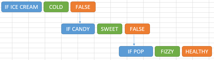
If we use real values, we could represent different inputs and outputs by this table:
| Input | Output |
| Ice Cream | Cold |
| Candy | Sweet |
| Pop | Fizzy |
| Apple | Healthy |
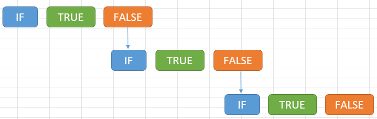
Or in psuedo-code
    If (Ice Cream THEN Cold)
    ELSE
    If (Candy THEN Sweet)
    ELSE
    If (Pop THEN Fizzy)
    ELSE
    Healthy
Notice that we don't need to explicitly test for the last input. If we have already tested for 3 of the 4 possible inputs and haven't yet found a match, then the final input must be the only remaining one : Apple, so the output must be Healthy.
You could visualize this in a diagram like so
Nested IF Builder
Looking at the Nested IF Builder we can construct the IF formula like this
I've only written the Nested IF builder so that we are replacing the False results with another IF. There's nothing to stop you replacing the True result with an IF, or using some other function for the True or False results.
If you didn't already, hopefully now you'll be able to understand how to do this yourself.
Note
I've used an old Excel 4 macro EVALUATE to calculate the result of the constructed formulae. I was trying to avoid using VBA. If you have any issues with EVALUATE not working for you, let me know and I'll work on a VBA version of the IF Builder workbook.


This was extremely enlightening
Glad it was helpful!
can anyone help me please? i am trying to make an IF formula for a different price depending on province
here is what i have but its not working:
=IF(N3=”ON”, “$5820″, N3=”AB”, “$5694″, N3=”BC”, “$1826″, N3=”MB”, “$1476″, N3=”QC”, “$3563″ , N3=”NS”, “$4686” )
Hi,
If you use IF then you need to nest another IF for each condition you want to test, like this
However it looks messy. If you can use the IFS function it’s a bit neater
Note that the values you are returning are text e.g. “$5820” not numbers so you can’t do any math with those. You should return numbers and then format the cell to display the leading $ sign
Regards
Phil
Please help, I need a formula for the following,
=if (A1=1, then A2 must equal sheet 2, A1) & (if A1=2, then A2 must equal sheet 2, B1) & (if A1=3, then A2 must equal sheet 2, C1) so forth, up to 12
Sounds like your data is in the wrong format if it’s spread across multiple sheets, but you need to reference them in one place. That said I expect you can’t change it easily, in which case simply write the formula using nested IFs, clicking on the relevant sheet and cell for each ‘must equal’ argument you mention.
If you get stuck, please post your question on our Excel forum where we can help you further.
Hello Mynda (and team)…
I was reading your most recent email newsletter (they are great BTW) and downloaded your “IF formula builder” to give it a try.
I am getting a “#NAME?” error in the “Result” cells for all the sheets. I think it is because of the use of the EVALUATE macro that you mentioned in the post in the “naming” of the “Result” named cells. Also, I am not familiar with the use of the @ in formulas (unless being used in or in reference to an Excel Table) – what is its purpose/function in this use case?
Has an updated version of the “IF formula builder” been planned and if so when will it be available?
Please advise; thanks.
Trevor
Hi Trevor,
Here is a good article about implicit intersection operator:
https://support.microsoft.com/en-us/office/implicit-intersection-operator-ce3be07b-0101-4450-a24e-c1c999be2b34#:~:text=Why%20the%20%40%20symbol%3F,same%20row%20from%20%5BColumn1%5D.
You have to allow macros to run, files downloaded from internet will have the MOTW (Mark Of The Web) and are usually blocked. To unblock a file, right click the file > properties, there should be a check box to Unblock.
With macros allowed, the macro 4 function Evaluate should work.
HI,
I am trying to build an excel file that I can use to help track patient visits. I have it set where there is an active or pending status, and if the status is active the next visit needs to be calculated from the last visit+the frequency set for a patient to be seen (Weekly, Monthly, Bi-weekly, Bi-monthly) and to even add more to the crazy layer if I could different colors show on the bars (red, yellow,green) to show whether a patient is past their next visit date, close, or within a week away from their next visit. Now if the status to begin with is left pending then everything I outlined above is null and left blank until its been made active.
ex. if status is active(column B), person 1(Column A) was seen on 12/30/2022(column D) and are scheduled at a frequency to be seen bi-weekly(Column C) so the next visit (Column E) will be calculated from last visit and frequency (Column C+Column D)
Hopefully this all makes sense
Hi Hayley,
Can you please upload a sample file on our forum?
Will be much easier to help if we see your data structure.
Hello Hayley,
This can be easily accomplished with data validation and a nested IF formula. The following is based on the column reference you mention.
Col “B” (status) – use Data Validation to only allow “Active”, “Pending”, or nothing.
Col “C” (frequency) – use Data Validation to only allow “Weekly”< "Bi-weekly", "Monthly" or "Bi-monthly
Col "D" & "E" – format cells as date (chose how you want it to appear; date must be entered as yyyy-mm-dd
In Column "E" use this IF formula: =IF(C2="Weekly",D2+7,IF(C2="Bi-Weekly",D2+14,IF(C2="Monthly",D2+30,IF(C2="Bi-Monthly",D2+60,""))))
Hope this helps you design the worksheets.
Hi,
My self Shankar
D/CJ8G0000444675/JCCR88FPZ472/64200AAN700US /000001/0000560.00/AAB/1/G/000/00
I need the after-4th / centenc in this data
will u pls help
Hi Shankar,
You can use the TEXTSPLIT function to split it into separate columns. Or if you have TEXTBEFORE and TEXTAFTER, you can use this formula:
=TEXTBEFORE(TEXTAFTER(A1,”/”,4),”/”)
Mynda
Thanks for your support
TEXT AFTER-TEXT BEFORE function is not available In my excel 13
Thank you’ll need to use the TEXTSPLIT function, or you can use this technique with the MID function.
Kindly help me create a formula for the below problem:
We now want to have a 9% price rise, so increase the prices in column D accordingly. HOWEVER there are some items (listed on the second tab in the Excel workbook) where we have already set a new sell price, and we want to use these prices, not the ones we have just calculated. Using a suitable formula in Column D, only add the 9% to the items NOT on the second tab, and if the code is on the second tab, still use the divide by 0.45, but don’t add the next 9%.
Hi Bryan,
This sounds a little like a homework question.
It refers to information and you haven’t supplied (the list of items on the second tab) so there’s no way to write an accurate formula without seeing that data. Please start a topic on our forum and attach your file so we can see if we can help.
Regards
Phil
I Am building a formula for factoring a score between 0 to 10 for the below
Threshold – 99.980%
Target – 100%
Achieved – 99.995%
Tentative Score – 7.5 as this score range is between (0 to 10) based upon achieved the score has to vary from 0 to 10
Hi Sarath, Please post your question on our Excel forum where you can also upload a sample file and we can help you further.
I am building an excel sheet but cannot get the formula correct. Tab1(Jan) ColumnB (Name), ColumnC (Tier)
On Tab Jan I need to pull – (Name Ben, Tier A) then (Name Ben, Tier B) then (Name Ben, Tier C)
I have 2 other people to do that for.
Last tab is the overview, the data is listed there.
Hi Abbey,
Can you please upload a sample file with your data structure and an example of the expected result on our forum? We will be able to help you much easier if we can see your data structure.
Thank you
Hi,
I have an IFAVERGAE formular, that needs to exclude ‘zeros>
I want to use this formula, but I get the error message, that I am using too many arguments. Do I need to put it in separate brackets?
=AVERAGEIF(Sheet1!D$1:D$400,E5,Sheet1!J$1:J$400,”0″)
Thx
Sven
Hi Sven,
Try this:
Mynda
Thank you, unfortunately, it did not fix the problem.
Sheet1 column D various items in a list
Sheet1 column J value for items related to column D
Sheet2 (the sheet I am working on, in column C I fill an item from Sheet1
Sheet2 column D I want to have the average value related to that particular item from sheet1, excluding zeros
For example, in Cell C3 I fill in an item, in Sheet1 columnD I have a variance of different items, D3 should now pick up the average value from Sheet1 columnJ related only to that item, excluding zeros.
In Cell C4 I fill in a different item and D4 should show the average value to that item only and so on…
Thx
Sven
Hi Sven,
Sorry, I can’t picture all that information in my head at once 🙂 Please post your question on our Excel forum where you can also upload a sample file and we can help you further.
Mynda
I enter the event date in cell E2. When dropdown event type in cell D2 is “Early”, I’d like cell H2 to display the date that meets this criteria, “The earlier of 29 days from event or 9 days after the end of the month in which the event occurred”.
Here’s the current formula: =IF(ISBLANK(E2),””,IF(D2=”Prompt”,WORKDAY(E2,5),IF(D2=”Early”,E2+29,IF(D2=”Optional”,””,E2+89))))
Thank you!
Hi RJ:
Mynda
I’m trying to If F2= (a drop down is located here with 31 different options) then G column will be a certain value H column will be a certain value and I column will be a certain value. All of these columns contain words.
For example:
F2 column (header- offense type) = Unsafe driving THEN
G2 column (header- escalation owner) = Billy Bob
H2 column (header- additional stakeholders) = Loss prevention, HR
I2 column (header- recommended escalation) = Coaching
Hi Alisha,
Please upload a sample file on our forum (create a new topic after sign-up), also provide what needs to be displayed for each value in F2.
If you have a table with 4 columns: column 1 will have those 31 dropdown options, columns 2-3-4 should have corresponding values for column G-H-I.
Formula for column G should then look like: =Index(Table1[Column2],Match(F2,Table1[Column1],0))
Formula for column H should then look like: =Index(Table1[Column3],Match(F2,Table1[Column1],0))
Formula for column I should then look like: =Index(Table1[Column4],Match(F2,Table1[Column1],0))
I know the client’s birthday (F3) and the report date (D1). If the client’s age as of the report date is between 61.0 and 62.0 I want to know their specific age and have it reported in cell N3, e.g. 61.40. If they are any other age I want the cell N3 blank.
(I have spent hours trying to figure out the formula for this. Any help is super appreciated!!)
Try this one:
=if(AND((D1-F3)/365>=61,(D1-F3)/365<=62),(D1-F3)/365,””)
if cell B5 IS EQUAL TO CELL F1 BUT LESS THAN D1 ENTER THE AMOUNT IN CELL F3
in F3
=IF(AND(B5=F1,B5
if value A1 greater than 300 then A2 multiply by 600 and if value A1 lower than 300 then A2 multiply by 400 in excel formula
Try:
=A2*IF(A1>300,600,400)
I want if the cell in a column is blank then move up till find a valve in column from bottom.
Try:
=Lookup(2,1/(A1:A100000<>“”),A1:A100000)
Hello- I’m stumped on how to accomplish the following:
If column E is ‘Negotiation’ I want column G to be column F+7
If column E is ‘Not Ready’ I want column G to be column F+360
If column E is ‘Project Completed’ I want column G to be column F+120
Column G and column F are dates. All help is appreciated!
-Ray
Hi Ray,
Try this in G2:
=F2+Index({7,360,120},Match(E2,{“Negotiation”,”Not Ready”,”Project Completed”},0))
I am a beginner with conditional formatting. My current issue is:
IF A2 contains “STRING” (within a longer text), then C2 = B2 + 5. Of course, this must be done for all values in A column.
Thank you very much for your help.
Hi Bogdan,
Try this where your text is in cell A3:
=IF(SEARCH("STRING",A3),B1+5,0)If you’re still stuck, please post your question on our Excel forum where you can also upload a sample file and we can help you further.
Mynda
Thank you very much for support. For unknown (for me) reasons the solution doesn’t produce any result. Even it was accepted (no errors) by Excel. I will post it on forum for a better analyse.
If D3:D22 = Y then it is 25 if it = N it is 0
Hi River,
You can only test one cell at a time e.g.:
Then copy the formula down to row 22.
Mynda
I am trying to create a formula that will have the values numbered 1-7 in a given cell in the column and the $ amount returned automatically that will correspond to that number entered. (each $$ after the initial $35 will increase by $15 ever time IE:
0 can be blank
1 would be $35 in the next column’
2 would be $50
3 would be $65, etc all the wayup through the highest quantity being 7
You should use VLOOKUP on a sorted list or XLOOKUP if you have Microsoft 365. Nested IF formulas are inefficient for this type of task.
Hi. I have been struggling with this for a year now. I still cant figure out how to work around it as there’s not enough excel expert working around me.. Please enlighten me with what I have been doing work with the formula
basically. I am trying to calculate project days in between 2 days. There’s:
A1 : 15 March 2020 -> 1st Starting date of Project
A2 : 25 October 2020 -> 2nd Starting date of Project
B1 : 31 August 2020 -> Project Deadline
C1 : 02 September 2020 -> today()
My Formula :
IF(DATEDIF($A1-1,$C$1,”md”)=0, IF(DATEDIF($A1-1,$C$1,”y”)=0,” “, DATEDIF($A1-1,$C$1,”y”) & ” years “) & IF(DATEDIF($A1-1,$C$1,”ym”)=0,” “, DATEDIF($A1-1,$C$1,”ym”) & ” months “) & IF(DATEDIF($A1-1,$C$1,”md”)=0,” “, DATEDIF($A1-1,$C$1,”md”) & ” days “), IF(DATEDIF($C$1,$A1,”md”)=0,” “,DATEDIF($C$1,$A1,”md”) & ” days remaining “))
What I want to find out is how long the project duration.. and if the project is overdue deadline, how long has it been due
I wanted to make it so that.. It will count the duration between the starting date and today(). Most of the time, the starting date is before the ending date.. But if the project have not start yet. I want it to count down to 0, and immediately continue to count the duration between the starting date and today().
And If the project have passed the deadline from the starting date, I want it to also immediately continue to count the duration.
This is all I wanted to make.. but I somehow cant get it right.
Someone please assist me with this formula
Hi Chiika, please post your question on our Excel forum where you can also upload a sample file and we can help you further.
hello i need help how to create a formula i have number criteria
: 200-290 -1B
300-790-2S
800 – 1250-1B: 1S
1260-2230-1B; 2S
2240-3090-1B-3S
3100-3390-1B; 4S
Here is the profile length in millimeters, if the profile length is from 200mm to 290mm I need to multiply it by 1B if the profile length is between ‘800mm and 1250mm I need it multiplied by one big bracket and one small, is it possible to create one formula for all these criteria and how it would seem
Hi Kestutis,
Sorry the problem is not clear. How do you multiply by a big bracket??
Please post your qs and attach a workbook in our forum, and provide examples of the calculations you want and the desired results.
Regards
Phil
I want a correct formula or which formula to use if in a excel sheet I column c7,d9,e4,etc, comes in sheet II row c5,d5,e5,etc,
If you just need to reference those cells, try simple cell reference:
-in cell C5 from sheet2, use this:=Sheet1!C7. Same for the rest of he cells you need.
If I misunderstood, please provide more clear details.
In cell F9, use an IF function to test if the value in D9 is less than or equal to 8. If this condition is true, then multiply D9 times E4 (the regular rate). If the condition is false, then multiply 8 times E4 and add to that E9*E5 (the overtime rate).
Hi Haley,
The syntax for IF is
=IF(Test, Result if Test is True, Result if Test is False)So what you have is
Test = D9<=8Result if Test is True = D9*E4Result if Test is False = 8*E4+D9*E4and putting that all together
=IF(D9<=8, D9*E4, 8*E4+D9*E4)Regards
Phil
I am trying to create a formula for a lot of numbers if
number >130 are called Platinum,
number >100 are called Gold,
number >70 are called Silver,
number >40 are called Bronze,
number <=40 are called Newbie.
Can anyone helo with the formila
Try:
=INDEX({“Newbie”,”Bronze”,”Silver”,”Gold”,”Platinum”},MATCH(A1,{0,40,70,100,130},0))
Hi! I’m relatively new to an indepth use to Excel so I’m looking for some help on building my first “if” statement.
I’m creating a receipt spreadsheet for my boss. The sheet will have multiple years on it (I’m trying to convince him to do a tab per year, but we’ll work up to that). He wants to have a box near the top of the sheet that has different columns (i.e. “meals”, “parking”, “admin”, etc) to identify the type of receipt with each item being identified in the actual list by a note (i.e. “vendor”, “location”, “amount”, “type”).
What is the best way to write an “if” statement that will pull the amount for a receipt “type” over to the correct “type” running total?
Thanks for your help!
Becky
So far I’ve got this written:
=IF([@Note]=”Meals”,J4=SUM)
but it says my syntax is wrong.
Hi Becky,
I’m not sure what you’re trying to do, but in English your formulas says:
If the value on the current row of the Note column contains the text ‘Meals’ then J4 equals SUM. I hope you can see that this doesn’t make sense. Perhaps you want to return the value form cell J4 if the value in the Note column contains the text ‘Meals’. If so, you need this formula:
If that’s not it, please post your question on our forum with your sample Excel file so we can see what you’re working with.
Mynda
Hi Becky,
Your boss is right not to want a separate tab for each year. This is the opposite of how you should structure your data in Excel. Please see this post on how best to structure your data in a tabular format. Then you can use a PivotTable to easily extract the data you want for your running total by receipt type.
If you go down the separate tab path you will only cause headaches for yourself going forward. I hope that points you in the right direction. If you’d like help with the PivotTable, please post your question on our Excel forum where you can also upload your sample Excel file.
Mynda
=IF(SUM(A3-A2)+2>0,SUM(A3-A2)+2,0)
Can you minimize this formula…
=MAX(0,A3-A2+2)
Hi. I’m trying to have a column tell me whether a row contains certain different values, if so put Open otherwise put No.
Values are: “T”, “PE”, “E”, “P”, “N”, “OFF”, “X”
I Had formula =IF((AND(R723=”T”, R723=”PE”, R723=”P”, R723=”E”, R723=”N”, R723=”OFF”, R723=”X”)),”Open”,”No”)
BUT it does not seem to work.
Please help
Hi Kimberly,
That cell R723 cannot have in the same time all those values, this is what AND means. Replace AND with OR and it will work.
I am trying to make a formula for my finances sheet. That adds all the values from a category AND times’ the USD transactions by 1.32.
What I have right now is
=SUMIF(E:E, “Groceries”, B:B)
So it checks what is in column E to see the category and then adds the value in column B. I need to add to the formula so it checks column C and if it is USD, it will *1.32 before adding.
Hi Meghan,
There’s a couple of ways to do this. You could use another column to calc your USD values and then modify the SUMIF to sum those values.
For example in Col C you would have the text USD in the cell (row) beside the US dollar values. Col D would then be =IF(C1="USD",B1*1.32,B1) and you would use =SUMIF(E:E, "Groceries", D:D)
Or you can use 2 SUMIFS, the first to sum the USD values only and multiply by 1.32 for the conversion, and the 2nd to sum the other non-USD values
=SUMIFS(B:B,E:E,"Groceries",C:C,"USD")*1.32 + SUMIFS(B:B,E:E,"Groceries",C:C,"")
Regards
Phil
I am trying to use a formula that will let me take the first 3 characters in a cell and if those three character are specific characters it will reference sheet 2 and take the information in that cell. So IF Left asd c1 will put in sheet2!a1 IF Left aft c1 will put in sheet2!a2 so on and so on.
Anything would be helpful! Thank you in advance!
Hi Aby,
You can use this
=IF(LEFT(C1,3)=”asd”,Sheet2!A1,IF(LEFT(C1,3)=”aft”,Sheet2!A2))
but if you have a lot of possible values for the first 3 characters of the string in C1, you might not want to nest a lot of IF statements.
Cheers
Phil
I am trying to fix a formula and/or make it work. It works somewhat but I’m having issues with it. I have a list of excluded holidays, however my formula is not excluding them from my dates. The formula is as follows: IF(COUNTIF($J$10:$J$23,Q18-7),IF(WEEKDAY(Q18,2)=1,Q18-10,Q18-8),Q18-7)
I have a date already calculated in cell Q18. I need the value in my new cell to calculate to one week prior, not on a weekend or holiday and if it falls on a weekend or holiday to back date to the previous week day.
Any help would be tremendously helpful!!!
Hi Jennifer,
Your first IF criteria doesn’t have a logical test, it’s just the result of COUNTIF. Please post your question and sample Excel file on our Excel Forum where we can see the formula in context and help you further.
Mynda
HI,
I am trying to work out how to put a formula in excel to pull the criteria through for the following,
spending customer after not spending for 12 months is classed as a new customer
So the last 12 month they have not spent then on the 13th month they have I would then like to enter “NEW”
I have entered the following formula but get an error.
=IF(AND(SUM(D10:O10)1,”NEW”)
D10:O10 is Jan to Dec sales – these are zero sales
P10 is January sales which the customer then started to but again
we would class this customer as new customer.
Can you help?
Hi Leeanne,
That said, this formula will need manually updating each month, so you’d be better to write a formula that will automatically shift one month forward. For help with that please post your question and a sample Excel file on our forum where we can help you further.
Mynda
Hi Mynda,
I have tried the above and get ‘the formula is missing an opening or closing parenthesis’
I have tried adding an ‘)’ but does not seem to work
I have been putting this as well
=IF(SUM(D4:O4)1,”NEW”)
Oops, I missed closing the AND. I’ve corrected it in my comment.
YOU ARE THE GREATEST OF ALL TIME! THANK YOU WITH EVERY BODY HEART!! YOU JUST DON’T KNOW HOW LONG I
HAVE BEEN WORKING ON THIS FORMULA! YOUR WORKBOOK IS FANTABULOUS!!!
No worries, glad it was helpful.
Regards
Phil
I am trying to see if it is possible to do a formula where if two cells AQ2 and AW2 have the letter x in them that it will place that same x in cell M2. But I also want it setup to where if there is not an x in AQ2 and/or AW2 that then the sum of I2+14 would show. These are all dates aside from the x of course. I have a spreadsheet when I track what is received and when it is due by. The cell for I2 is showing the date in which I received the first item which then projects for two other items to be due within 14 days of the date in which I received the first item. I want that date to remain until those two other items are received and then an x to be placed showing that those two things have been received once I mark them off in their own unique cells. I hope that makes sense.
Hi Kayla,
Try this formula in M2:
=IF(AND(ISNUMBER(SEARCH(“x”,AQ2)),ISNUMBER(SEARCH(“x”,AW2))),”x”,I2+14)
Thank you, I tried that and while it did not give me an error for the formula, when I tried to put an x in AQ2 and AW2 it did not place an x in M2.
Hi Kayla,
The formula expects an x in both cells, only then it will return an x. Make sure the calculation is set to automatic, there is no reason for the formula to not work. You might have to retype the double quotes used in formula, when you copy the formula you usually get a different char for double quotes.
What if I wanted to update the formula so that some cells could have “x” or “na” entered in it but the tracking cell I would still want to then kick back either an “x” showing it is done or the date–showing when it would be due?
Hi Kayla,
Please provide more details, not sure what formula you are referring to.
Sorry, I had meant I wanted to update my original formula I discussed on this thread originally in October 2019. It would be the same exact situation except I want to add in for the formula to search for ‘x” and “na” whereas currently it only searches for “x”.
I am trying to see if it is possible to do a formula where if two cells AQ2 and AW2 have the letter “x” or “na” in them then it will place an “x” in cell M2. But I also want it setup to where if there is not an x in AQ2 and/or AW2 that then the sum of I2+14 would show. These are all dates aside from the x of course. I have a spreadsheet when I track what is received and when it is due by. The cell for I2 is showing the date in which I received the first item which then projects for two other items to be due within 14 days of the date in which I received the first item. I want that date to remain until those two other items are received and then an x to be placed showing that those two things have been received once I mark them off in their own unique cells. I hope that makes sense.
Try this one:
=IF(ISNUMBER(MATCH(AQ2&AW2,{"xna","nax"},0)),"x",I2+14)
Hi,
I need a formula that will meet these criteria:
Cell A consist different characters such as 45657852, 54631326, Location, Bike.
i want to create a formula to get those characters start with numeric 4, 5 as inventory and rest as Non-Inventory in Cell B.
Hi Sanjay,
I’m not clear what you mean by ‘get as inventory’. Can you please be specific about the actual outcomes you want and provide examples. Please open a topic on the forum and supply a workbook containing data and your expected results.
Thanks
Phil
Hi,
I thought this would be simple but I can’t get it right.
I need a formula that will meet these criteria:
If cell A is Routine and cell B is => 5 days this is a “pass”
If cell A is Routine and cell B is 2 days this is a “pass”
If cell A is Urgent and cell B is =”Routine”), AND(L2>=5),(OR(E2>=”Urgent”), AND(L2>=2), “Pass”, “Fail”)
Can anyone advise please?
Thanks,
Steve
Something got lost when I pasted this in. I’ll repost.
Hi – I need some help. I want to calculate for each month the amount of times the Letter E, M or R comes up. example in January I have 2 E’s, 2 M’s and 3 R’s. How would I write the formula so I am able to do this for each month. I assume it would be a separate formula for each Letter in the Rank Range. I am a basic Excel user and have been trying to figure this out.
Rank Jan 2020 Feb 2020
E 1.0 1.0
M 1.0 1.0
E 1.0 1.0
M 1.0 1.0
R 1.0 1.0
R 1.0 1.0
R 1.0 1.0
E 2
M 2
R 3
Hi Paul,
The commend has lost the formatting so it’s a bit tricky to understand the layout of your data, but you most probably need to use the COUNTIF or COUNTIFS functions.
If you’re still stuck, please post your question on our Excel forum where you can upload a sample Excel file with your data and desired result.
Mynda
Bravo! Well done. One of the best demonstrations for learning the IF formula, particularly the extremely powerful AND, OR and XOR forms of the IF function and the section about the EVALUATE formula is a great reminder of some of the handy “old” features hidden in Excel that still work today.
Thanks Thomas.
What is happening on the “Data Validation” tab?
Hi Ron,
Not sure what you mean by ‘what is happening’? It’s got the values for the Data Validation lists on it.
Regards
Phil
Thanks for this helpful IF Formula Builder
1) Although the name Result1 refers to =EVALUATE(‘IF Builder’!I7) in the Name Manager, I am getting always #Value!
2) Where can I find the code?
Hi Emmanuel,
There is no code to look at for this. The issue may be that the in your locale you use something other than a comma as the separator between function parameters.
If you use a character other than a comma, edit the formula in the Formula Created cell and replace the comma with your locale specific separator. I know in other countries they use a semi-colon.
Regards
Phil
Thanks for the post. My learnings from this are less to do with the formula syntax but about how to reference cell addresses in formulas, your very clear nested if maps and how to use EVALUATE and other older macros.
You’re welcome Stan
(take 2)
COOL TOOL!
I really like this addon. It will definitely go on my “must read” and “recommended” list.
Here are a few observations / suggestions (I hope you find some useful)
– remove the blank columns between the input areas to make it easier / faster to enter their data
– use colors to highlight the output areas where they are not supposed to type
– make the blank column between the input and output areas wider, to make the separate functions clearer.
– Add headers above input and output areas
– Color code the sheet tabs to make them more visible
– add a TOC page to make navigation to the example pages more obvious
– it looks like you have not finished the Data Validation tab in the file I downloaded.
– consider putting the test data area below the code generation area. That way they don’t have to worry about copying too many rows of data and accidentally overwriting your examples. I understand people find it easier to work with A1 than A#
– just curious, in the AND/OR tab, did you apply manual background colors in the input areas, especially the “Result if True” cells?
– on the Nested IF tab, consider stacking the 3 conditions vertically, or indicate subsequent tests if false, ie “Test 2 If Test 1 FALSE”
– explain your color code, ie BLACK fill means no data entry
– If you could extend the tool to include table examples that would be great. At first attempt I don’t see how. At minimum, include an example of a table formula to explain why tables are so great.
Here is a link to an example of your file I tweaked a little: https://1drv.ms/x/s!Am8lVyUzjKfpnxAYPpc4v89AAHyZ
Keep up the GOOD WORK!
R.
Thanks for the suggestions Rohn. I’ll have a look at your file.
Regards
Phil
Philip,
I’m confused about a few things in the workbook.
1) You mentioned that you used an Excel 4 macro, EVALUATE. I don’t find in the workbook the EVALUATE function being used anywhere, nor do I find a macro named EVALUATE.
2) There IS a single macro, in the “IF Builder” Worksheet_SelectionChange. What is this macro used for?
3) In your RESULTS boxes, each one ends with something like “Result2&T(NOW()))”. What is the purpose of the T(Now()) in the formula?
Hi John,
If you open the Name Manager you’ll see that there are some names that reference the EVALUATE function. If you read the post on Excel 4 macros it explains more.
Oops, I forgot to remove that Worksheet_SelectionChange macro. I wrote that when I was developing the workbook and forgot to remove it. I’ve removed it now so it should be gone from any subsequent downloads of the workbook.
The Result2 is one of the names I referred to that you’ll see in Name manager. When developing this workbook I found that the EVALUATE function wasn’t always recalculating when I changed an input. So the &T(NOW()) bit is a trick to force recalculation. Because NOW() is volatile it will recalculate every time you change something on the sheet and hence force the entire expression to be recalculated. The T function returns a string if the input parameter is a string, otherwise it returns an empty string. So &T(NOW()) appends an empty string to my result. I force the Result to be recalculated, but I don’t affect the value of the result because I’m appending an empty string to it.
Cheers
Phil
Great presentation of these formulas. It helps to figure out what’s behind the curtain.
Living in Québec, I’m using french Excel. I had to change a few things to make it work. Translating the name of the functions was needed.
The only thing I can’t figure is the formulas in the K column. I get #VALEUR! as a result. It seems the EVALUATE function doesn’t work. Probably a translation problem too.
Thanks Jean-Sébastien,
Thanks for fiddling about with this to make it work in your locale. With regarsd to the #VALEUR! error, check the Name Manager and see what Result1 refers to. It should be =EVALUATE(‘IF Builder’!I7)
Regards
Phil
what is T(now()) in the “Results” formula
Hi Steve,
When I was putting this together I found that the EVALUATE function wasn’t always recalculating when I changed an input. T(NOW()) is a trick to force recalculation. NOW() is volatile and will recalculate when you change something on the sheet. This forces the entire expression to be recalculated.
The T function returns the input parameter if the input parameter is a string, otherwise it returns an empty string.
So &T(NOW()) appends an empty string to my result. I force the Result to be recalculated, but I don’t affect the value of the result because I’m appending an empty string to it.
Cheers
Phil
When opening the file, under ‘Result” only “#VALUE!” appears, and not the expected result. The formula is ‘=IF(OR(A7=””;B7=””;C7=””;E7=””;G7=””);””;Result1&T(NOW()))’.
Hi Geir,
Open the Name Manager and check what the name Result1 refers to. It should be =EVALUATE(‘IF Builder’!I7)
Regards
Phil