Using a Formula Instead of VBA

Sometimes we get requests to provide a VBA solution to a problem. But when we look at the problem, VBA is not the best answer, using a formula is.

What this tells me is that people don't know how to use Excel's functions and when they come up against a problem they think is difficult, or just don't know how to solve it, they go looking for a VBA solution.

By making yourself familiar with basic functions like IF and VLOOKUP (just to name two) you can make your life a lot easier.

Function or Formula?

You'll often see the terms function and forumla used interchangeably. Strictly speaking however, a function is the actual piece of code written into Excel's core programming that gives you a result based on inputs you give it.

For example, IF is a function but when you use it like this

=IF(A1>10,True,False)

you've written a formula using the IF function.

How Does IF Work Again?

Let's go over how the IF function works before we get any further. It really is very simple and can help understand how other functions work too.

The syntax is IF (Test_Condition, Result_If_True, Result_If_False)

where Test_Condition is some test that can be evaluated to see if it is true or false e.g.

• A1>10 : Is A1 > 10?
• A1*0.5=A2 : Is A1 x 0.5 equal to the value in A2?
• A1>=A2 : Is the value in A1 greater than or equal to the value in A2?
• A1="Hello" : Does A1 contain the string "Hello"?
• AND(A1>0,A2<10) : Are both of these conditions true? Is the value in A1 greater than 0 AND is the value in A2 less than 10?
• SUM(A1:A10)>1000 : Is the SUM of the values in cells A1 through to A10 greater than 1000?

Easy. So once we have our test, IF will determine if it is TRUE or FALSE. If it TRUE then the result returned by the IF function will be whatever you specify in Result_If_True.

If the result of your test is not TRUE then the result of the IF function will be whatever you specify by Result_If_False.

Result_If_True and Result_If_False can be things like a number, a text string, a Boolean Value or even another function. For example:

=IF(A1<=10, SUM(B1:B5), SUM(C1:C5))

means that if the value in A1 is less than or equal to 10, then the result of this IF formula will be the SUM of the values in cells B1 through to B5.

If the value in A1 is greater than 10, then the result of this IF formula is the SUM of the values in cells C1 through to C5.

Now we've covered that, let's look at some examples of where formulas are better than using VBA.

Download The Workbook

All of the problems I'm about to describe, and their solutions, can be found in the example workbook you can download here.

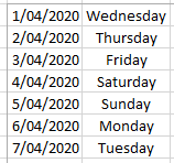
Get the Day From a Date

Given that we have a series of dates, how do we get the day of the week i.e. Monday, Tuesday etc?

I was asked to work out a VBA solution to this but all we need is the TEXT function.

=TEXT(A1,"DDDD")

gives us the day of the week

and if we specify a different format we can get the abbreviated day of the week.

=TEXT(A1,"DDD")

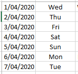
The TEXT function allows us to format numbers (which is what dates are) in specific ways.

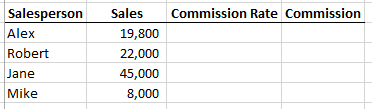
Work Out Commission Rate and Commission Based on Sales

We have a number of sales people and we want to work out their commissions based on how much they have sold.

The commission rates based on sales are

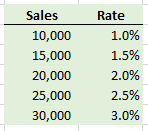
The original question had a lot more salespeople and commission rates and I think that was the reason a VBA solution was requested. That and the logic required to work out commission based on various sales bands.

Your first thought might be to use IF but as you have to allow for many sales bands, you have to nest a lot of IF functions and that can get very messy and confusing.

All you need is VLOOKUP.

VLOOKUP allows you to look up a value and return an adjacent value.

So we can lookup a value in the Sales column and return the adjacent value from the Rate column.

In the image below, the formula in C3 is looking up the value in B3 from the range F3:G7. It matches against the first column (Sales) and returns the adjacent value in the 2nd column (Rate) of the range F3:G7.

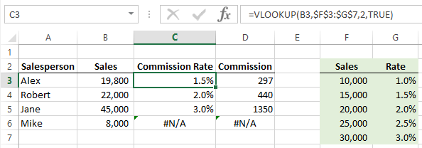
But the Sales amount in B3 is 19,800. How does VLOOKUP know what to do because our sales bands don't have this exact value?

That's where the last parameter we're supplying to VLOOKUP comes in. By specifying TRUE we're telling VLOOKUP to give us the nearest, lowest, value that matches what we are looking for.

So the nearest, lowest, value to 19,800 is 15,000 so we get 1.5% returned.

To do this you must use VLOOKUP with a sorted list which in this case means having the Sales bands sorted in ascending order.

You can get VLOOKUP to do exact matches too by specifying FALSE for this parameter but that's not what we want here.

What if someone sells less than $10,000 worth of widgets? We don't have a value that VLOOKUP can return in this case so there are two ways to deal with this.

Add a value of 0 with 0 commission to our lookup values

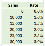
Any volume of Sales below 10,000 will now result in 0 commission.

Or wrap the VLOOKUP in an IFERROR function.

=IFERROR(VLOOKUP(B22,$F$22:$G$26,2,TRUE),0)

If we now ask VLOOKUP to lookup a sales value less than $10,000 it will cause an error but our IFERROR will catch this and give us a 0.

What started off looking like a complicated problem that required VBA was solved just be using VLOOKUP (and IFERROR).

Finding a Haulage Firm Based on the City and Store

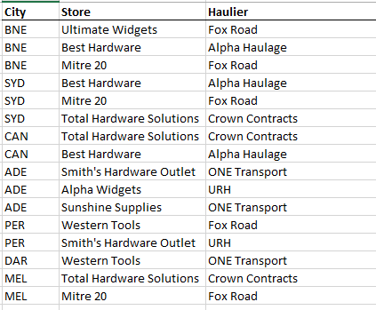
Our company sells widgets and we supply various stores across the country. The company we use to transport our widgets depends on what city and what store we are shipping to.

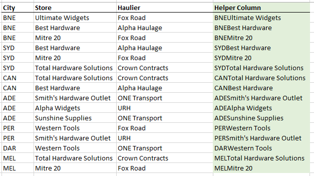
Here's a list of the cities (3 letter abbreviations), stores and haulage firms

What we want to do is to enter the city and store and have the haulage firm shown in another cell.

I'm using Data Validation in the City and Store columns to allow me to choose from drop down lists.

This is a little more complicated but if we break it down into steps, it becomes manageable.

The essence of what we are trying to do is lookup a value (the haulier) based on two other values (the city and store).

You could write a monstrous nested IF but as soon as you have more than a few IF statements it becomes very unwieldy and you should stay away from doing that.

We could possibly use VLOOKUP but if our data layout is fixed so we can't insert another column before (to the left) of the Haulier column, we can't use VLOOKUP because it can only return values to the right of the lookup column.

There is a way to use the CHOOSE function with VLOOKUP to do lookups to the left but I will not use that method here.

I'm going to use INDEX and MATCH.

The key here is that we need to create a helper column which consists of the city code and store name joined together. What this means is that we are effectively looking up two things at the same time.

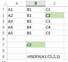
INDEX returns the value at the intersection of a row and column. So if we write =INDEX(A1:C5,2,3) the result is the value at Row 2, Col 3 in the range A1:C5.

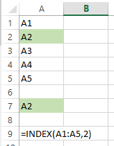
The column can be omitted so writing =INDEX(A1:A5,2) means we are looking up the value in just one column (A1:A5) and we want the value in Row 2.

Because each combination of city code and store name is unique, the Helper column is filled with unique entries meaning we can use INDEX to look up where a particular combination of city/store occurs.

But how do we do that dynamically so that we aren't specifying a hard coded number? By using MATCH.

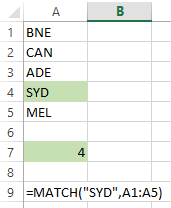
MATCH returns the relative position of a value in a list (a column or row).

If I write =MATCH("SYD",A1:A5) with the sample data below, the result is 4.

By using MATCH to lookup the position of the values in the Helper column, we can then feed that into INDEX which returns the corresponding value (from the same row) from the Haulier column.

In the image below, the formula in C2 is =INDEX($H$2:$H$17,MATCH(A2&B2,$I$2:$I$17,0))

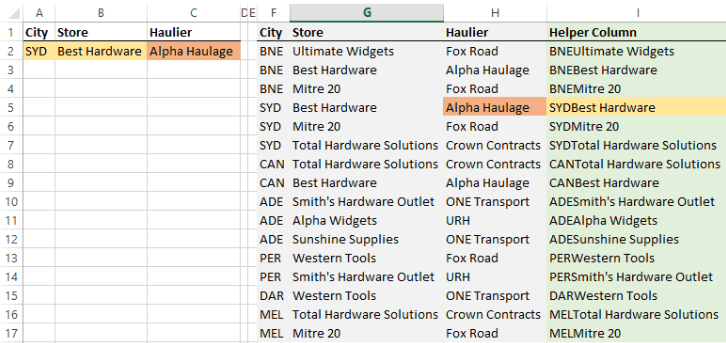
We use MATCH to lookup the joined strings in A2 and B2 which is SYDBest Hardware and we get the result 4.

MATCH(A2&B2,$I$2:$I$17,0)

This 4 then indicates to INDEX which haulage firm to return =INDEX($H$2:$H$17,4) which gives us Alpha Haulage.

Why Don't People Use More Functions/Formulas?

Don't get me wrong, VBA is great if you need to automate repetitive or boring tasks, and you need VBA to do certain things that you just can't do any other way.

But knowing the functions available to you in Excel and how to use them in formulas can save you a lot of time pursuing other avenues looking for an unnecessarily complex solution.

Part of the problem is just not knowing what functions are there and what you can do with them. You need to take the time to learn them.

That might seem like a boring, waste of time to familiarise yourself with functions you aren't going to use right away, but in the long run it's so useful.

When I was first starting out in I.T. I remember reading a book on the DOS prompt and all it could do. I used to do a lot of batch scripting and it helped me immensely. I became the guy people came to when they needed help with their scripts.

Thing is, I didn't know any magic. I'd simply taken the time to learn how to use the tools I was using. And it wasn't hard.

If you aren't familiar with Excel's functions, you should make the effort to learn what they can do.

Not only will you get your work done more quickly, your confidence in using Excel will soar.

This is precisely why you should look at our Advanced Formulas Course.

Advanced Formulas Course

The course is designed to get you quickly up to speed with the functions that are going to give you the biggest efficiency gains.

Many of the functions are considered advanced, but when you’ve finished the course you’ll realise that everything is easy once you know it.

The course uses real world examples and covers both the fundamentals for each function and less obvious uses for them. It's these more advanced techniques that will really set you apart from the crowd.

Check out the Excel Formulas Course now.