At first glance the Excel TEXT function appears quite limited. Its purpose is to convert numbers to text in a specific/custom format.
There are two key points here:
- The numbers become text. This means you can’t use them in any math type of formulas.
- On the upside you can format the numbers anyway you want…almost!
Hold up!
Why would you want to convert a number into text when it means you then can’t use that number in any math calculations/formulas?
Wouldn’t you just format the cell with the number format you want?
The answer is ‘yes’ most of the time, but I’ll show you a clever use for it in a moment.
Excel TEXT Function
First, the syntax is:
TEXT(value, format_text)
Where the value is the number or reference to the cell containing the number you want to format, and format_text is the format you want, enclosed in double quotes.
Download Workbook
Enter your email address below to download the sample workbook.
Let’s look at some examples.
Excel TEXT Formula Examples
Example 1 – Format as a Currency.
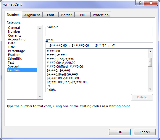
If you don’t know the character codes to use you can refer to the Format Cells dialog box (CTRL+1 to open it) to get the number format ‘code’ (that is the $#,##0.00 part) you need:
You can use any number formats for the format_text argument that you find in the Format Cells dialog box under the ‘Number’ tab.
Or you can write your own custom format.
If you're new to custom number formats check out my comprehensive guide to custom number formats.
Example 2 – Formatted as a date with hyphens instead of the Excel standard forward slash.
Note: 41640 in cell A5 is the serial number for the date 1st Jan 2014. More on understanding dates in Excel here.
Example 3 – Display day of the week.
Again we’ve taken a date in cell A6 and with the TEXT function we’ve only displayed the day of the week. If you wanted to display the full name of the day you would use “dddd”.
Example 4 – Add leading zeros to a number.
This is handy for invoice numbers or other numbers/codes that require a leading zero.
Limitations of TEXT Formulas
As I mentioned at the beginning, the above examples all convert the numbers in column A to text in column B.
Examples 3 and 4 are ok formatted as text (the day of the week and leading zeros) as they are unlikely to ever be used in a math formula so having them as text won’t cause you a problem.
But it’s not ideal for examples 1 and 2 (format as currency and date), as it’s likely you’ll want to perform a calculation using those numbers at some point in your worksheet’s life.
A better option for examples 1 and 2 is to just apply the number format to the cell in column A.
Combine Text and Numbers in One Cell
I think the best use of the TEXT function is to use it to combine text and numbers in one cell.
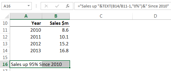
As you can see in cell A16 below:
In the formula bar you can see I’ve used the ampersand symbol (&) to combine the text, “Sales up” and “Since 2010”, with the number returned by the TEXT function, which I've formatted as a percentage:
="Sales up "&TEXT(B14/B11-1,"0%")&" Since 2010"
Which results in one text string:
Sales up 95% Since 2010
You’ll notice in this example I’ve also performed a calculation for the value argument of the TEXT function, which is then formatted as a percentage:
TEXT(B14/B11-1,"0%")
Which results in:
95%
The benefit of using a formula for the value argument is that any changes in the data will automatically be reflected in my statement in cell A16.
Bonus Trick
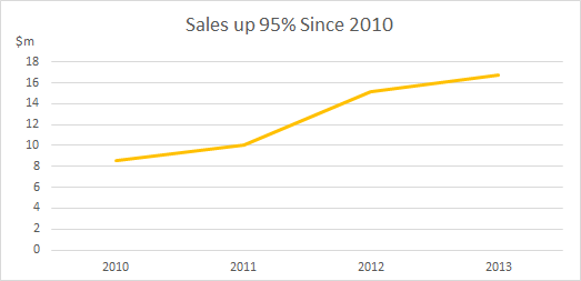
Now you can link cell A16 to your chart title and not only will the chart update if the numbers change, but so will the title:
To link the chart title to cell A16:
- Left click the chart title to select it
- In the formula bar enter = then click on cell A16
- Press ENTER
Crazy TEXT Function Trick
At the very beginning I said the TEXT function converts a number to text which means you can’t perform any math calculations on the results.
However, in this video Mike Girvin, of Excel Is Fun, shows a crazy trick (at 3:30) with the TEXT function to convert a date into the right format. Even MrExcel doesn’t believe it will work:
Explanation: in the video Mike performs a calculation on the text function which in turn converts the value in the cell back to a number.
Similarly, you can also convert a cell containing a text function back to a number by multiplying the cell by 1, or add 0, or use the VALUE function, to name a few.
Note: There are some limitations to this. For example you can’t convert the text 'Wed' in example 3 above back to a number, but you can for the other examples.


No worries about dealing with TEXT() results being text representing numbers so long as the facts on the ground do not make the following bearable to enter. With the thought above of a column of invoice values to add up, it would work like a champ:
{=SUM(VALUE(J1:J7))}
43 individual things to wrap like that in disparate places in the workbook, years later, well, yeah… unbearable. I prefer formatting the cells though, as suggested since it is more directly on the problem.
For Lee’s question, just below (I’m sure he sent it in and was answered, but someone reading here woudn’t see the answer he got), an IF() test using ISBLANK() would achieve what it seems he wants:
=IF(ISBLANK(A1),””,TEXT(A1,”#,##0.00″))
(just picked a format, of course). Works for true blanks (“nulls”) and sort of blanks like =”” creates.
If a cell in column A is empty, can you make the formula return a blank cell for the TEXT function as I am struggling with this for some reason.
Hi Lee,
I’m not sure if the cell in column A is empty it’s the same as a blank cell. Can you please give me an example of what you mean?
You might like to post your question on our Excel forum where you can also upload a sample workbook.
Mynda
Excellent instruction – So clear and precise.
Now what about aligning text boxes in a chart that are setup vertically on right side of chart as column. I am in Dashboard course with Avg Cost numbers on right side of chart, and am unable to align them.
Thanks, Allen 🙂
You’ll find the alignment tools for text boxes in the ‘Drawing: Format’ tab of the ribbon which is active when the text box is selected. So, select all of your text boxes that you want to align, then in the Format tab: Arrange group use the Align tools.
To select multiple text boxes just select 1 and then hold down SHIFT to select more. You can also select 1 and then press CTRL+A to select all objects, then you can unselect the ones you don’t need by holding down SHIFT while you click on the ones you don’t want.
You might also like this free add-in from Excel Campus that allows you to
use arrow keys to align the chart elements
Mynda
Thanks for the great article! That’s one crazy trick that Mike Girvin figured out.
This is one format I use quite often to convert dollars to millions.
=TEXT(A4,”$#,##0,,.0″)&”M”
Cheers, Jon.
You can also add the ‘M’ inside the formula like this:
Kind regards,
Mynda.