I’ve put together this Excel custom number format guide as a resource for our members. There are loads of ways to apply custom number formats and as a result I find myself answering questions that are covered in this post on a daily basis.
To be clear, number formatting in Excel is used to specify how a value should appear in a cell or chart, but it doesn’t alter the underlying value that you can see in the formula bar. Unless of course you format a number as text, in which case it can no longer be treated as a number in math formulas.
Download the Cheat Sheet & Workbook
Enter your email address below to download the cheat sheet and example workbook.

Table of Contents
- Excel Custom Number Format Guide
- Download the workbook
- Applying Custom Number Formats
- Number Format Structure
- Hiding All Values
- Hiding Zero Values
- Custom Number Format Characters
- Literal Characters
- Special Characters
- Digit Placeholders
- Thousand Separators and Scaling
- Currency Formats and Parentheses for Negative Values
- Using Symbols in Formats
- Colors
- Date Characters
- Time Formats
- Fractions
- Percentages
- Scientific Notation
- Text/Labels
- Color Code based on Values/Conditions
- Repeating Leading and Trailing Characters
- Padding with Zeros
Applying Custom Number Formats
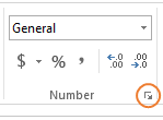
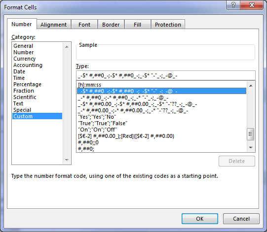
To apply a custom number format first select the cell or cells you want to format, then CTRL+1 to open the Format Cells Dialog box, or go to the Home tab and click on the arrow in the Number group:
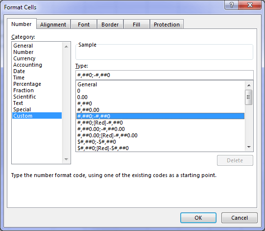
This opens the Format Cells dialog box in the Number tab (below), where you can choose ‘Custom’ from the Category list and insert your format in the ‘Type’ field:

Number Format Structure
Let’s start with the anatomy of a number format.
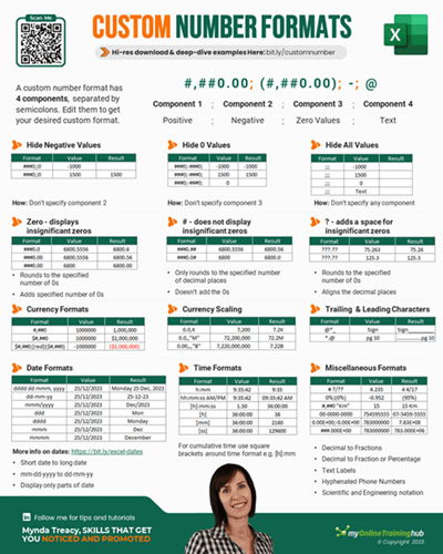
A number format is made up of 4 components, with each component separated by a semi-colon:
Component1;Component2;Component3;Component4
- Component1 formats the POSITIVE value
- Component2 formats the NEGATIVE value
- Component3 formats ZERO values
- Component4 formats TEXT
In other words; POSITIVE ; NEGATIVE ; ZERO ; TEXT
Note: spaces around semi-colons above are added for clarity but are not required in the format.
You may be familiar with number formats you find in the Format Cells dialog box, like this:
In the above example only the positive and negative formats are specified, in which case the zero format will be the same as the positive format and text will be formatted as it was entered.
In fact when we omit components Excel behaves as follows:
- When just one component is provided with no semi-colons in the code, Excel will check to see if the format is one of the default ‘Number’ formats and revert to that format. Otherwise, if the format is unique then all numbers will be formatted according to the format provided.
- When the first two components are provided Excel will use the same format for zero, and text will appear as entered.
- When the first three components are provided Excel will use the formats specified, and text will appear as entered.
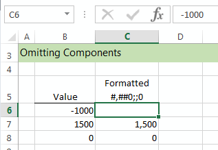
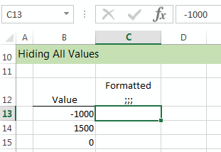
- If any components are skipped or left blank e.g. in this format the negative component has been skipped, #,##0;;0 and so the negative value will not display as demonstrated below:
Hiding All Values
When all components are omitted and just the 3 semi-colons specified, Excel will not display anything in the cell. It’s a clever way to hide data in cells and charts.
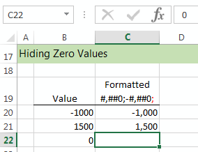
Hiding Zero Values
Another common question is ‘how do I hide zero values from displaying in my chart labels’. The answer is simply to use the technique in point 4 above and omit the format for the zero component. See the example below:
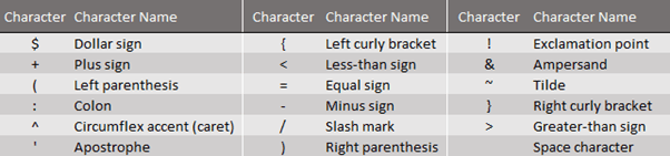
Custom Number Format Characters
You may have noticed custom number formats that contain unusual characters like this:
These characters are used as codes to tell Excel how to format the value. Let’s look at them in turn.
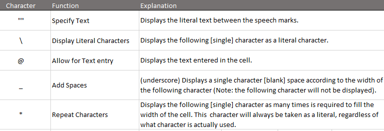
Literal Characters – these appear as entered in the custom number format:
Special Characters – define how other characters are treated
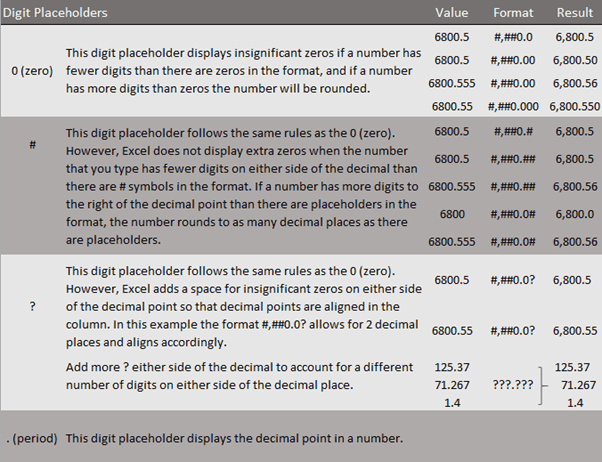
Digit Placeholders – used to control how numbers that contain decimal places are displayed:
Thousand Separators and Scaling
The comma is used to display the thousand separators in a number when it is enclosed in # signs or by zeros, and when it follows a digit placeholder it scales a number by 1000.
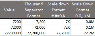
Tip 1: We can scale a value to millions by using two commas, as you can see in the example in the last column above. And for billions we add 3 commas.
Tip 2: When appending ‘K’ for thousands we simply type it in the format, but ‘M’ for millions must be entered with a preceding \ as the example above, or inside double quotes. This is because ‘M’ is already reserved as a character for the date formats. More on date formats soon.
Currency Formats and Parentheses for Negative Values
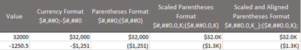
Tip 1: In the example in the last column above I’ve used the underscore and right parenthesis to align the decimal places. You can see them in red in the number format here: $#,##0.0,K_);($#,##0.0,K)
Remember the underscore is a special character that adds a space according to the width of the following character, in this example the right parenthesis.
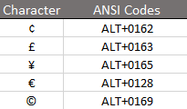
Tip 2: if you don’t have a particular currency key on your keyboard, you can enter it into the Custom Number Format dialog box using the ANSI code. To enter an ANSI code, hold the ALT key and type in the 4 digit number. Here are some example ANSI codes that might be useful:
Using Symbols in Formats
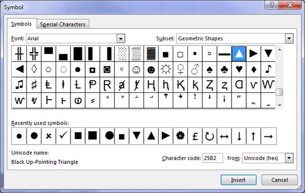
Alternatively, you can use the Symbol tool (Home or Insert tab) to find the character you want and then insert it into a cell. From the cell you can copy it to your clipboard and paste it into the Custom Number Format dialog box.
Tip: You can also insert symbols like up or down triangles, just make sure they’re the Arial Geometric Shapes (subset) variety and not Wingdings:
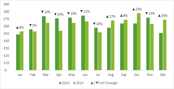
For example, this format displays positive percentages with an upward facing triangle and negative values with a downward facing triangle.
▲0.0%;▼0.0%
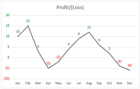
Symbols can be quite effective when used in reports or charts like the one below:
Colors
We can specify a color for a format, for example you might like to format negative values in red. Color formatting is done in one of two ways:
- We can use the color name surrounded by square brackets, like so:
$#,##0.0,K_);[red]($#,##0.0,K)
Which results in negative values like this: ($1.3K)
However, with color names we’re limited to these:
[black]
[green]
[white]
[blue]
[magenta]
[yellow]
[cyan]
[red]
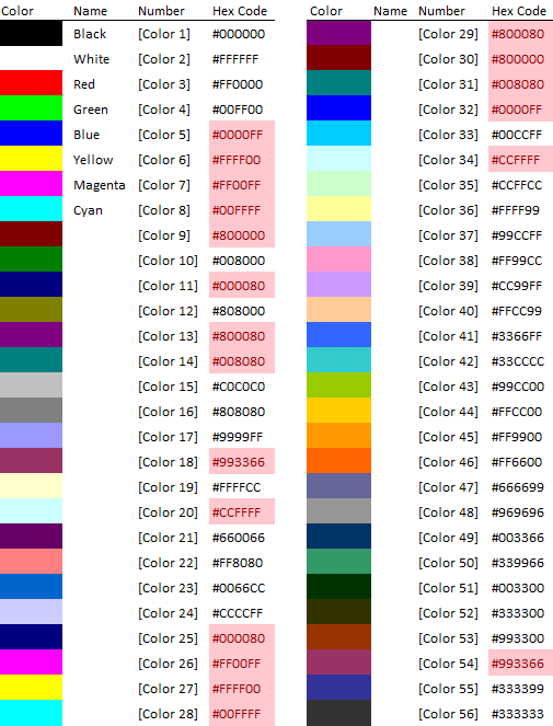
- Alternatively we can specify a color index number e.g.:
$#,##0.0,K_);[color 3]($#,##0.0,K)
Using the color number opens up a total of 56 different colors, although 5 of them are duplicates, as you can see by the hex codes in red below:
Tip: Apply color formats to chart axes or labels. Note: if you have labels then you don’t also need the vertical axis or gridlines, unlike my example below:
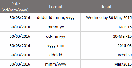
Date Characters
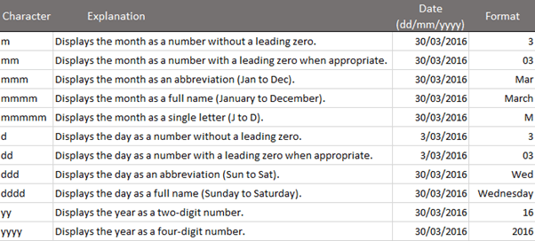
We can combine the month, day and year characters together in various configurations to get the desired format. Here are a few examples:
Click here for more on how dates and time are handled in Excel.
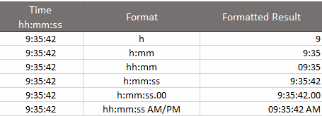
Time Formats
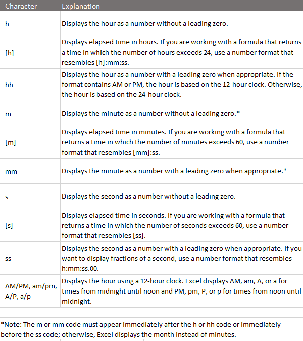
Just like the date characters, we can combine the time characters to get the format we’re after. For example:
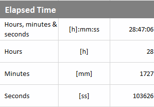
And when we’re adding time that exceeds 24 hours, or 60 minutes, or 60 seconds we can display the elapsed time like so:
Fractions
Let’s go back to school and recap some of the different types of fractions:
- Proper – where the absolute value of the fraction is less than 1 e.g. 1/2
- Improper – where the absolute value of the fraction is greater than or equal to 1 e.g. 4/3
- Mixed Fractions – are another way to write improper fractions where the whole is written separate to the fraction, for example 4/3 would be written 1 1/3
Use the ? symbol to specify the varying number of digits to display.
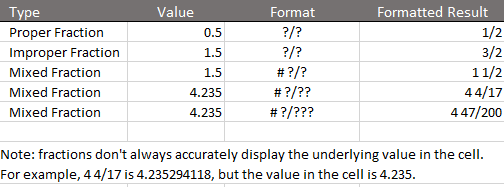
It’s important to remember that the underlying value in the cell, as displayed in the ‘Value’ column above, is what is used in your formulas that reference those cells. The Formatted result is simply how it appears, but you must be careful if you are using those formatted results in calculations that don’t reference the cell directly. For example if you were to enter those formatted values into a calculator you’d get a different result to a formula that referenced that cell.
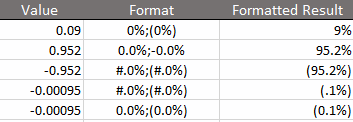
Percentages
Use the % sign to display numbers as a percentage of 100. Remember, a zero in the custom number format displays both significant and insignificant digits, and the # will only display significant digits as per the examples below:
Scientific Notation
Scientific Notation allows us to express very large numbers in a decimal form of shorthand. It’s commonly used by scientists and mathematicians. Let’s use 7,830,000,000 as our example value. I think you’ll agree it’s a pretty big number.
In scientific notation we can express it as 7.83 x 10⁹
We raise 10 to the power of 9 because 9 decimal places have been removed from the original number to be left with 7.83. And when we multiply 7.83 by 109 we get our original value of 7,830,000,000. Ok, math lesson over.
In Excel (and some calculators) we can’t use ‘x’ in a number, nor can we insert superscript. Instead we use the upper (or lower case) E+ notation like so:
7.83E+09 or 7.83e+09
To apply this formatting the custom number format is 0.00E+00 or 0.##E+00.
Remember we can use 0 to display both significant and insignificant digits, or if we only want to display significant digits we use #.
Here are some examples:
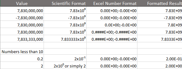
Did you notice the precision in the ‘Formatted Result’ of the 3rd example above? See how it appears to round the value to one decimal place and therefore omits the ‘3’ in 7.83. Be wary of this if you’re likely to refer to the face value of these cells, as opposed to the actual underlying value.
Remember to use the 0 digit place holder to show both significant and insignificant digits, and use the # to only display significant digits.
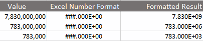
Engineering Notation
Engineering notation is a version of scientific notation in which the exponent of ten must be divisible by three. The format contains 3 # before the decimal place and 3 zeros after the decimal place to force the result to return an exponent that is divisible by 3.
Text/Labels
We can append or prefix our values with text while still maintaining the underlying number for use in formulas. This can be handy when formatting values like kilometres or days/hours/minutes, Over/Under etc.
To display both text and numbers in a cell simply insert your text in double quotes, or if it’s only a single character then precede it with a backslash (\).
*Don’t forget, Literal Characters are displayed without the need for quotation marks.
Here are some examples you might find useful:
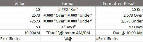
The last example uses the @ symbol for Text. In other words, the cell is formatted as text, which is also why it is left aligned, but the custom cell format displays the # tag at the front of the text without the need to actually type it in the cell.
Color Code based on Values/Conditions
Remember that by default the custom number format is broken into the following components:
Positive ; Negative ; Zero ; Text
However, we can override the default components with up to two conditions and add color coding based on criteria we set.
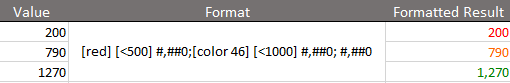
For example, let’s say we have a threshold of 500 units per day. Anything below this should be red and anything 500 or above should be formatted green. We can use the format:
[red] [<500] #,##0;[color 10] [>=500] #,##0
Which yields the following results:
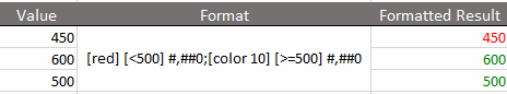
Tip: once a condition is met Excel doesn’t test the other conditions so it’s important you get the order of tests correct so it doesn’t stop at the first criteria. Just like a nested IF formula.
Of course we could also write this format like so:
[color 10] [>=500] #,##0; [red] [<500] #,##0
What if we want 3 conditions? Well, we can’t insert 3 conditions as such, but we can insert 2 and then apply a font color to the cells, which will be picked up for all remaining values. This works because custom cell formats override the font color.
In the example below values less than 500 are red, values less than 1000 are orange/amber and values 1000 and over, for which there is no criteria, pick up the cell font color, which is green:
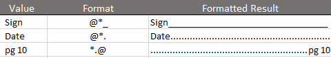
Repeating Leading and Trailing Characters
We can fill a cell containing text values with a specific character using the asterisk symbol. For example:
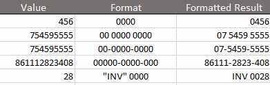
Padding with Zeros
Remember that zero is a digit placeholder which displays both significant and insignificant digits, so we can exploit this to force Excel to display an insignificant zero at the front of a value, or to apply spacing between digits.
It’s handy for phone number formats, bar codes, product codes etc. Here are a few examples:
Notes on Custom Number Formats
- Custom Number formats are saved in the workbook in which they’re created and are not available in any other workbooks.
- Custom Number formats do not change the underlying value. This is important if you want to reference those cells in formulas.
- Formats can appear to round values which will not be reflected in the results of formulas that reference those cells
- Regional Settings – this post assumes your region uses the full stop/period character for a decimal place and a comma for the thousand separators. If your region differs, please amend accordingly.
Sources
I’d like to recognise the following resources which I learnt from in the writing of this guide:


First of all thank you for all your guides. “Repeating and remembering are the same thing just in reverse.” Always nice to stay up to date and recall you as resource.
Even though a rare case: if you are ranging multiple magnitudes of numbers (p, n, µ, m, 0, k, M, B, T) you could write a function combining it with a Lookup-Table.
Could be used for Finance or Technical measurements or Dashboard Templates where you are unsure about the Magnitude of numbers (consumption per year vs consumption per minute).
=LET(
Value; AD16;
Scale; ROUNDDOWN(LOG(ABS(Value);10)/3;0)*3;
Format; “##0.0”;
IF(Scale>=-2;
TEXT(Value;Format&REPT(“’”;Scale/3)&XLOOKUP(Scale;Table3[Scale];Table3[Unit]));
TEXT(Value/(10^Scale);Format&XLOOKUP(Scale;Table3[Scale];Table3[Unit])))
)
Unit Scale
0
K 3
\M 6
\B 9
\T 12
\m -3
µ -6
n -9
p -12
Thanks for sharing, Thorsten! Not sure I’ll have a use for it, but it’s an interesting idea that I’m sure some people will find useful.
Greetings Mynda,
and thanks very much for the resources your provide us. Your T-Shirt is apposite.
The following extension of one of your examples may prove useful to others.
I needed a custom format which would display the number in the cell as an amount in Euro if it was less than 36526 (i.e. 1 Jan 2000), and as a date if it was above or equal to that (i.e. after 1 Jan 2000); the font colour etc. should remain at the default. Your example lead me to try this:
[>=36526];[>=36526];dd.mm.yyyy
and it does just what I wanted it to; Thank you!
Thanks for sharing, Chris. I edited your post to display the greater than character. It wasn’t displaying because it’s used by HTML on the webpage as code, so you have to enter it using the HTML code for the greater than sign.
Hi Mynda,
Just reading this after returning from Christmas /New Year break.
On the Hide values section you don’t mention the use of the format “;;”?
This hides only numeric values.
Format Value Result
;; Text Text
Thanks for sharing, Gordon!
Will be very useful. Thanks.
Great to hear!
is it possibel to put Percentage number in brackets, Ex:
the increase from 50 to 100 is 50 (50 %)
What is the VBA codes to put “50 (50%)” in one cell?
You can’t duplicate a number in a cell, but if you just want brackets, you can use this format: (0%), but keep in mind, brackets are universally used to indicate a negative value in financial reporting. Another option is to use the text function to convert the two numbers to text and then concatenate them e.g.
=TEXT(A1, “#,##0”)&TEXT(B1, “(0%))
If you get stuck, please post your question on our Excel forum where you can also upload a sample file and we can help you further.
Hi,
I use custom number format #.##0__________ to align on decimal points without showing a decimal point when it is not needed. But I can’t seem to combine this with a currency symbol? Is that possible?
Hi Koen,
Have you tried adding the symbol?
_-$ #.##0__________
This is GREAT!
Great to hear it was helpful 🙂
How do you freeze the output of your custom format so u can move them to another workbook while retaining the final output?
Not sure what you mean by freeze, Tricia. You can copy and paste formats only via the Paste Special menu.
I created a comment moments ago about an issue I had, literally after closing page, realised i can use conditional format by doing Between 0.1 and 1.1 custom format as 1. Sorted.
ref: =SUM(IF(FREQUENCY(MATCH($L$1,$F25:$K25,$L$1),ROW($F25:$K25)-ROW($L$1)+1)=1,1))
6×7 Cells are preformatted to custom as 00:00:00.00 (HH:mm:ss.00), If time is entered it would return a 1 in the last column, but if someone stuck in 1 in the cells the cells would display 24:00:00.00 which still counted as one in last cell of row, but looked crazy being 24:00:00.00. So the above conditional format has solved my problem.
Glad you figured out a solution, Steve. If we can help in future please post your question on our Excel forum where you can also upload a sample file and we can help you further.
I have table 6 columns x 7 rows and one column on the end for countif, when time is entered into any cells in the row, then cell at the end of table row returns 1.
each row is counted as one test and each column is for entering the data corresponding to what device was timed – So if more than one device was used for that test, it still counts as one test.
=SUM(IF(FREQUENCY(MATCH($L$1,$F24:$K24,$L$1),ROW($F24:$K24)-ROW($L$1)+1)=1,1))
The format of cells is custom, 00:00:00.00, so time is HH:mm:ss.00 when entering stopwatch data.
I then use each cell at the end of table rows that contain 1 to do a count up of how many
tests were done.
The problem I have though is that some people just put 1 in the cell to say that the test was done. by doing that, it shows as 24:00:00.00 – which although works for the final count of tests, it makes it look like that test took 24:00:00.00 to do.
Is there a way that if someone does put in a 1 instead of time, to still be counted / behave in the same way as time so that I can still do the count of tests and the 24:00:00.00 isn’t displayed, 1 is instead?
Thank you in advanced
Or is there a way that I use ‘If’ function to format cells as number, time, text, etc?
So if 1 is entered then it’s a 1 if not, then just keep as time entered.
the article does not include custom locale/different languages (eg for month names) formatting available in custome formatting..
Hi Tomas, you might find this tutorial helpful: https://www.myonlinetraininghub.com/excel-dates-displayed-in-different-languages
Problem accumulating days
Hello I have time records in general format “0.000000” and I transform them with “dd hh:mm”, but this works as long as the numbers are less than 32.
For example “3.456789” with “dd hh:mm” results in “03 10:57”.
but if I apply “33.456789” with “dd hh:mm” results in “02 10:57” (due to the haul of the month).
How can I do this with numbers greater than 32?
Hi James,
Displaying elapsed time in days, hours and minutes in Excel is explained here.
Mynda
Hi
I have a question about custom format cell , Which codes or characters in custom format cell should I use that when I copy a formula from another cell and past in formatted cell then the result of formatted cell (displayed number) does not change and main as before pasting?
Hi Arash, the formatting doesn’t dictate whether formats are retained upon pasting or not. If you want to copy the formatting when you copy a cell you simply press ENTER to paste it. By doing this you are copying the whole contents of the cell; formula, formatting etc. when you press ENTER.
hello, thanks for your help
Suppose we have a table where the third column is the product of the first column multiplied by the second.
a b a*b
2 3 6
6 3 18
5 4 20
3 5 15
3 6 18
2 7 14
Then we change one of the cells of the third column using the custom format cell and the character “apple” as follows.
a b a*b
2 3 6
6 3 18
5 4 20
3 5 apple
3 6 18
2 7 14
Now if we copy the second row cell of the third column and paste it in the fifth row cell of the third column, the word apple changes to the number 15.
My question is what character instead of “apple “ to use in the custom format cell that does not change the word apple after copying the second row of the third column and pasting in the fifth row of the third column?(for example add the characters “#*., @ and etc. with apple may be was the answer)
Hi Arash, it’s not the formatting it’s the pasting you need to alter. If you paste all by pressing ENTER to paste then the format from the second row will override the format in the 5th row. It doesn’t matter what format was previously in row 5, you’re replacing it when you paste the data from row 2. If you want to retain the format in row 5, then you must use Paste Special > Values.
Thank you for your guidance ,Mynda
But that was not what I meant. In fact, I might ask the question, is it possible to define a format for a cell that contains a number that when we paste a formula into it , the number does not change in the cell ?
Hi Arash,
Let’s say you want a cell to always display the number 10 despite what is entered into it. You could use this custom number format: “10”
If you then wanted to copy and paste a cell containing a formula into the cell with the format “10” you would have to paste as special > formulas.
Note: if you performed a math equation on the cell formatted with “10” it would ignore the 10 and only read the underlying value/formula result contained in the cell.
Mynda
This one is in error: The symbols are reversed.
===
For example, this format displays positive percentages with an upward facing triangle and negative values with a downward facing triangle.
▼0.0%;▲0.0%
===
Well spotted, David! Fixed now 🙂
Is there a way to combine letters and numbers? For example, I know that I can create a custom format, AA-#### which will return AA-1234. But I would like to create a custom format that would include an unknown letter. Example, AA-1234B. The last letter would change with data entry.
Hi Lori,
I’m not sure how this last letter would be entered as such. Please post your question and sample Excel file on our forum where we can help you further: https://www.myonlinetraininghub.com/excel-forum
Mynda
Hi,
I found the topic interesting.
However, I cannot find an explanation of why excel shows a number below zero in this way “375,647,372,869,797,000.0”. It is a result of a formula, but for other results I have 1 decimal.
Thanks.
Hi Monica, please post your question on our Excel forum where you can also upload a sample file and we can help you further.
It is because Excel will only keep the first 15 digits in a number if handling the entry as a number.
Nowadays, it will automatically format the entry as a text string. If you then convert it to a value (perhaps =VALUE(cell) might be how it happens), it again only keeps the first 15 digits.
It CAN, however, display plenty of 0’s after those digits. This is how you end up with your example value… it trims off everything after digit 15, then pads it with 0’s to match the entered length.
One guesses other entries, the ones you get a single decimal place with, are rather shorter than this example.
Hi there,
I was wondering if anyone can help me. I am trying to change numbers into phone numbers ( with their correct prefix)
I have a column of numbers, with the + sign , when I go into the ‘number’ – ‘Format Cells’ – ‘Special’ – I have no special text her to change into phone number?
Can anyone let me know if there is something I need to change, I have been googling all morning to see what I can do, but all that seems to come up is to use this method to change into phone numbers,but of course I cant.
Any help would be great.
Thank you.
Hi Sarah, if your number already has a + sign prefixing it, then it’s text and you cannot apply a custom number format to text. Please post your question and sample Excel file on our forum where we can help you further: https://www.myonlinetraininghub.com/excel-forum
Hi Mynda,
The article was great and covered a lot of options for Custom Fomatting. Some new tips were available in the comments.
One thing I needed to know was how to convert to different comma placings. In some countries there is a comma as follows : $ 37,230,555.22 is written as Rs. 3,72,30,555.22. Is it possible to define the custom format with a different comma placement. Putting a 0\,00\,00\,000.00 does the job, but is there a proper way with # & $ because as soon as I change the currency to Rs. Hindi it starts showing the 00,000,000.00 format.
Appreciate your help
Hi Sandeep, I’m not an expert in different locales, but Excel is designed to format dates and numbers according to the locale settings in Windows and Excel. If you change the currency by selecting the currency format, then you are also changing the other parts of the format, as opposed to just replacing Rs. in your custom format with the Hindi currency symbol. Mynda
Hi Mynda,
One would think it should but the Currency format just changes the currency symbol from “$” sign to the sign for Rupees.
But does not change the other parts of the format.
I think I will go with the option that I had earlier.
Thanks anyway
An interestiing thing about Excel is that it does NOT make all available custom formatting options available out of the box.
Options that are used in languages/cultures other than English can be very useful. Japanese, for example, has many options with dates…
So installing something like Hindi might (or might not… I am not experimenting) bring to you the kind of number formatting you need. As mentioned below, that may not be a panacea. But it seems almost certain Excel adjusts to their customers in places like India if only because they figure there could be LOTS of them in a country that populous.
I found this out when adding Japanese as an available language. I will not casually suggest you add a language like Hindi (perhaps) as it happens that the language just added will take primacy from the start and you have to have the path to switching back to English (or whatever you start with) laid out already if you don’t know the new language… not pretty… And then one confronts the fact that I cannot find a way to remove an available language.
Why remove one? Well, because options are available and one might set formatting using one but if it is from the extraneous language, no one working with you’s Excel will have the ability to render it. So… looks great on your computer, but your boss can’t figure it out. “Oh, hey boss, you gotta make this particular whole language available in your Excel. Yeah, yeah, right, and then get your boss and his boss to do so too.”
Hard conversation to figure will work out for you!
I have a column of 1000 #s that are whole numbers and need to be changed to decimals.
Example : 1017000 need it to be 10170.00. I know you can format them I just can’t get the formula rite. Can you help?
Hi Ryss, This isn’t a format, this is dividing a value by 100 to make it a smaller value. You can do this with paste special. In an empty cell type 100. Copy that cell then select the cells you want to convert > paste special > select Values and Divide.
Mynda
Hello
Some of my cells filled with numbers end with asterisk. I’d like to custom format everything like 0,?????;-0,????? [so commas in one line and up to five decimal places], but can’t find any way to apply this formatting system to those cells with asterisks. Could anyone help with that?
Marcus Elivetti
Hi Marcus,
If a numeric value includes an asterisk then it is text and cannot be formatted with a custom number format. You need to remove the asterisk from the cell. Perhaps you can put it in an adjacent column.
Mynda
Hello, Mynda
Thanks for your answer.
Actually I can’t do that, they need to be kept, as additional columns would spoil whole the table.
Now I’m thinking of a formula to remove asterisks where they are and conditionally format those cells as having the asterisk added via \* [all those cells have numbers ‘larger than..’ or ‘smaller than..’], but I can’t cope with large distance between a number and *, which, on the other hand, destroys commas vertical alignment..
ME
I am trying to do the 10-digit number (original: 3035559876) and I am trying to change it to 10-digit numbers like (333.555.9876) like a phone number. I kept putting the # and space but I want to (.) decimal in between just like the one above.
You need to use the back slash to force the custom number format to display the period as a literal character. You can use this custom number format:
000\.000\.0000
Mynda
Thanks a Lot , Fundamentals explained with great clarity, lucid details with examples
for our clear and quick understanding
Thanks Vipul
I use the following format for my management accounts (rounded to nearest £’000)
#,##0,_);(#,##0,);-?
Anything that is actually 0 is expressed as a ‘-‘ but anything that is rounded to 0 becomes ‘0’ and makes the report look untidy.
I don’t want to change the actual values (e.g. MROUND function) as this introduces rounding errors in balance sheet etc.
Grateful for any suggestions. Apols if already covered but I could not see it.
Fabulous resource – keep up the great work.
Hi Casey,
Simply replace the zeros in the format to # i.e.
#,###,_);(#,###,);-?
Mynda
Hi Mynda. Thanks for your response. This has has just replaced the ‘0’ with a ‘blank’ whereas for any amount between 499 and 0 (or -499 and 0), I need to it to show ‘-‘ without changing the underlying value. Can send a screengrab if that helps. Thanks! Casey
Ah, sorry. It can’t be done. I would suggest that if you have values as low as that, you should add decimal places to the rounding instead e.g. #,##0.0,_);(#,##0.0,)
No problem and thanks.
I believe the following custom formatting string would do what you desire:
[>1] #,##0,_) ;[<-1] (#,##0,) ; -?
(Although I might misunderstand your application and therefore not be too helpful.)
Making a separate Comment for the way I usually (admittedly, not "often" in quantity, but in all such cases) use thing that allows the above.
Very clear guidance. But I still haven’t figure out my issue. I want to custom format when i enter value, it has bracket. example value= 12.22, result= (12.22). I figured this out, but have problem when value=0.32, result=(.32) when I want it to be (0.32)
Please help me with this
Hi Sarah,
The format should be:
(0.0#)
Mynda
Very useful guide. Thanks.
I’m looking for a way to display numbers up to two decimal places in normal notation (e.g. 0.12) and smaller numbers in scientific notation (e.g 0.000012 as 1.2E-5). Is there a way to do that?
L.E.:
I ended up accomplishing what I wanted using conditional formatting, but I’m still curious to know if there is a way to do it using some kind of creative number formatting.
Hi,
In excel, the custom format has 4 sections we can use:
2. Negative values
3. Zero values
4. Text values
“1;2;3;4”
There is no switch to evaluate the cell in order to choose what format to apply, only with conditional formatting you can do that, as you already did.
The following string should work:
[>0.01] 0.00 ;[<-0.01] -0.00; 0.##E+00 ; @
Unable to format date
We’d love to help, but your comment doesn’t give us anything to go on. Please post your question in our Excel forum where you can also include a sample Excel file.
Hi!
How can I add zeroes to the right of a number to make it 4 digits making it a bigger number rather than not changing its value? for 123 to 1230 and not 123 to 0123.
Thank you so much in advance.
Hi Al,
A custom format will not do that.
Your numbers are integers? Or there will be decimal places?
Hi Al,
If you want to append a zero to all of your numbers, you can format them with this:
###”0″
Note, it will make 123 display 1230 and 1234 will display 12340
The underlying numbers will still be 123 and 1234 respecively.
Mynda
Hi, then if the time custom format as below is what means?
[0][h]:mm
Thank you
That’s not a number format Excel recognises.
[0][h]:mm;
That isn’t valid either.
I have a series of reports, all starting with the same 8 numbers (05171007) then the report number 0001, 0002, etc. How can I format the number cell to display 05171007.0001, 05171007.0002 by just typing “1” and “2”, respectively.
Hi Joe,
Use this custom number format: “05171007.”0000
Mynda
Hi Joe,
Use this custom format: “05171007.”0000
Scientific Notation almost: How to I format “3.14159” as “0.314159E+01”
I require this text string (8/15/2019 6:30:00 PM) to be formatted as a proper date in excel. Neither formatting the cell nor using the DATEVALUE function seems to work. is there a way to do this, or is it just that the format of the text is incompatible with DATEVALUE?
8/15/2019 6:30:00 PM needs to be 2019/08/15 18:30:00
Thanks in advance…
Hi Paul,
The problem is the date is formatted as text, instead of a proper date serial number. Also, if your regional settings are dd/mm/yyyy then Excel will struggle with the date because it’s in a mm/dd/yyyy format. You can use Power Query to fix the date format, if you’re familiar with Power Query, or try some of these techniques to convert the text date to a proper date serial number.convert the text date to a proper date serial number.convert the text date to a proper date serial number.
I suspect you’ll either need to use Text to Columns to separate the date and time portions into their own columns, then add them back together in a formula. If you get stuck, please post your quesiton and sample Excel file on our Excel forum where we can help you further.
Mynda
Thanks much, Mynda. The incompatible text was, as suspected, the root of the issue. Text to Columns is a fairly straightforward approach. Will do that.
Is there a way that I can change the format for AM/PM to match my company’s brand standard as a.m. or p.m.?
Hi Cheryl,
Just put AM/PM after your format, like: h:mm AM/PM
Hi there
Thank you for your resource, very helpful.
I do however have one question I hope you can assist with or point me in the right direction.
I have cells in an excel workbook which are number formatted as Accounting or Currency. The numbers appear like so $180,00.40. However, when I click on the cell it reads 180319 and no longer has the dollar sign, decimals or comma. Can you advise on how 180319 would be able to reflect the number formatting (dollar sign, comma and decimal) in the formula bar as I am unable to mail merge this information across to Microsoft word as it pulls the actual sell value rather than the format that has been applied.
Hi Lauren,
In Excel cells, you can apply number and date formats to numbers, but in that cell it will always be a number, and a number you will see in the formula bar.
If you want to have text in formula bar, you need to have text in the cell, not numbers. Use TEXT function to convert numbers to text: =TEXT(180000.4,”$###,#.00″). In this case, cell content will be text, but in formula bar you will see… the formula. Type the format you need.
You can accomplish this by pulling the info from Excel into Word and having Word apply the number format. You are adding a Field in Word to obtain the info, and you can wrap that existing Field in another Field which does the formatting.
While that WILL do the trick, very likely the Field you currently use will allow you to format a number inside it and so not need the Field wrapping it to do the formatting.
I haven’t moved info from Excel to Word in decades, even when I should, so I cannot say for sure about the last part, but in ALL cases, the wrapping of that Field in a Field dedicated to formatting any number values will work.
Hi Mynda,
This is a GREAT article! Thank you for sharing your expertise!
Question for you… Is there a way to save custom number formats in Book.xltm so they’re available in all of the new workbooks that I create? I don’t want to save Book.xltm with “pre-formatted cells,” but I’d like the custom number formats to be available in the custom number list, if or when I need them.
For example: I created five different custom number formats in five cells in a worksheet. Those new formats are now available in my Number > Custom List. I deleted the contents of those five cells and reset their format to General (or, Clear All). The five custom number formats are still available in my Custom List. I saved the workbook as Book.xltm in my XLSTART folder. But, when I open Book.xltm, or start a new workbook, the custom number formats no longer appear in my Custom List.
Do I need to create new “Cell Styles” for the custom number formats to be permanent? I’d experiment with this, but my computer is out for repair. Thanks.
Hi Steve,
There is no easy way to store custom formats to be available in any new books. You can use a code in your Book.xltm that applies those formats to some cells of the active workbook. The code can be attached to a button in Book.xltm ribbon, to apply the format to selected cells. It’s even faster than going through the normal menu.
Is there a way to format the number as below:
1) =1000 and =1000000 and =1000000000 format as billions i.e. B
and
if the resultant number is less than 100 show the decimal value otherwise no need of decimal.
Eg:
33.5 should be 33.5 itself
345.6 should be 346
5655000 should be 5.7M
56550000 should be 56.6M
565500000 should be 566M
Thanks in advance
Hi Guru,
You can’t do this with custom number formats. You’d have to use a formula like IF(A1<1000000,A1,IF(A1>1000000,ROUND(A1/1000000,1),IF(… etc. to round the values depending on their size.
More on the IF Function here.
Mynda
You missed one time code, decimal values for thousandths of a second ie
sss.000
This format code is needed for precise duration and interval calculation. I found that this custom format works best for me
d “days” hh:mm:ss.000
Good reference for custom data formats. A few more examples would be nice.
(even for events that you count in just seconds.)
You have to enter your times as 00:00:00.000
Unfortunately Excel converts the time display in the formula bar to a date/time stamp starting at 1900-01-00 00:00:00 AM The decimal seconds are there, just not displayed in the formula bar.
The problem I have is I want to record elapsed time
Thanks for sharing, Ron.
Very useful.
Glad you found it useful, Sandeep 🙂
Muito bom o artigo, simples e objetivo, resulta muito no aprendizado.
Thanks, Samuel. Glad you found it useful 🙂
You mentioned “Thousand Separators and Scaling” for big numbers (kilo and mega).
what about little numbers (milli, micro ,piko)?
Hi Ofir,
Great question! There’s no custom number format for these. You’d have to normalize the numbers, as described here: https://excel.tips.net/T002928_Engineering_Calculations.html
Mynda
Hi Mynda
I have subscribed to a number of your courses and continue to be impressed by your flaws delivery. I also teach Excel in Lagos, Nigeria and find myself resorting to “err”s and “emm”s whilst trying to find the best way to put a point across.
FLIGHT DURATION ACROSS TIME ZONES
I recently found myself in a situation where I needed to prepare a spreadsheet of my journey which involved crossing time zones.
The usual “arrival time – departure time” gives erroneous results unless modified in the following way:-
At the heart of the solution is the fact that Excel views time in fractions of 24hrs so you would need to convert the difference in hours between the two time zones into a fraction of 24 then add or subtract this from the departure time in the formula above e.g.
Depart LON (GMT) 07:00 arrive LOS (GMT+1) 14:00
Flight duration = Arrival time – (Departure time + 1/24) = 6 hrs
Warm Regards
Shmuel
Thanks for your kind words, Shmuel!
Good of you to share your tip, too.
Cheers,
Mynda
This is a great article, Mynda! It got me wondering about what would happen if you changed the color palette (because almost all my old templates use a custom color palette). It turns out that the color codes for Color1-56 CAN be changed. For example, [Color10] doesn’t always have to be green. You can go to File > Options > Save > Colors and modify the color palette.
As another side note, the Color1-56 codes in Google Sheets are fixed colors (but match the default Excel color palette), so it doesn’t look like customizing a color will translate into Google Sheets if you upload/convert your customized Excel file.
Cheers, Jon. Great tip about the custom color palette. I didn’t know about that.
Mynda
It is really amazing efforts. Do you mind if I translate your post to Arabic along with the example file with keeping all the credit to you and your website?
viaexcel.com (website field is not working in comment area).
Thanks, Hussein.
Yes, you’re welcome to translate my post with a link back to my site for credit.
Cheers,
Mynda
Thanks Mynda for your permission.
Very usefull tips especially when combined with Excel cells styles. I’ve just read the article and it’s already saving me a lot of time. Thanks you so much for this !!
Thanks, Amadou 🙂
Hi Mynda
one of my favourite formats is when I want to show all numbers with the units in line, negatives in red (for screen viewing) and in brackets (for printing).
For this, I use #,##0.00 ;[Red](* #,##0.00) and, because I frequently use it, I’very made it into a macro and saved it in my personal sheet so that it available in any worksheet I use.
There was some fantastic examples in yours that I never even realised that I wanted to use before seeing them
Thanks for noting all of this down.
Thanks for sharing your tip, Simon. It’s always nice to hear what other people find useful and I’m sure there are more who will like this format too.
Mynda
Hi Mynda,
I released several year ago a similar workbook with a presentation to explain and illustrate the custom formating however I never imagine to use symbols to illustrate the grow of a metric like you done for charts. This tip is very interesting and this is what i love from MVP simple tips that make a big difference. Thanks a lot Mynda for sharing this.
Best regards
Mehdi
Thanks, Mehdi! Glad you found a new tip amongst it all 🙂
Well, you moved the bar for “pillar” posts. Let’s just call this a “foundational” post! I learned quite a few new tricks, some of which are eye-popping. This will be my go-to guide for formatting numbers!
Cheers,
Mitch
Thanks, Mitchell 🙂 Glad you’ll be able to make use of it.
This guide is a great tool, the kind I like to save for future use. Is there a better way to save it for offline use than a .PDF? The challenge with printing it to .PDF is the banner ads are still there and they block the guide.
Hi Bill,
Thanks for your email. We’ve added a ‘print’ icon to the left side of the page above. Unfortunately it bunches up some of the images a bit but it’s the best we can get it.
Kind regards,
Mynda
Mynda, that works just fine. Thanks for the help.
Hi Bill,
In Mozilla, you can view the page in “Reader View” (this option is towards the extreme right of the URL bar. In Reader View you get to see only the article minus all the ads and sidebar items. You can then either print a .pdf file using any of the free pdf conversion utilities like CutePDF, PDF-Viewer, etc., and save the pdf file to your system for offline use.
Well done for keeping this to such a short article; it really is a HUGE topic!
a few additional points to confabulate your readers further (and there’s more!)
Using a number formatted as text as a number – can be done if you add a double minus before it to force excel to evaluate it
Full year can also be formatted by using “e” instead of “yyyy”
Line feeds can be added to a format using ANSI code 10 (ALT+0010) – but dates will still show as ###### if the column isn’t wide enough (use the TEXT function if this really bugs you)
If you use a condition then the next rule is still used for negative numbers and the next for others (eg [<-1] -0;0.0;-0.0 will apply the -0.0 format to all zeroes and positives)
Colouring text using conditional formatting trumps number formatting (the two condition limit in normal formatting can be annoying)
Great tips, Jim. Thanks for sharing them.
On your condition example, just to clarify for others; it works that way because you only have one condition, my examples have two conditions.
Ah, and the subject DID come up.Even better! This is the Comment I alluded to earlier in the Comment chain.
You can use up to two conditions. BUT, you can still get a third one in if it is amenable to being used. For example, say you want Blue if >40, Red if 40]0 ; [Red][40, Red for >30, Green for >20″ which is sad.
Also, the conditions seem to have to come first or it fails to accept it. But it makes sense for that to be done (just not that it be required).
So you CAN get all three things done in many cases, but not always.
Thanks, Roy. Good to know. And thanks for all your contributions to the questions on this blog. Very helpful and much appreciated.
Sorry folks, the Comment has a bit missing in the middle.
For the first part, >40, 40] ; [Red][40, Red if 40, Red if >30, and desiring Yellow if <20. Since there would be an infinite number of results, like, say, 27, that the first two parts don't format, one could not be sure that making the third part Yellow would ONLY format those results that are 90, Green for <65, and Blue for the third part so anything from 65–90 would show as Blue. The key isn't the single value my example set up, but rather that anything between the two extremes be desired to be the third color.
My word, that’s all a terrible mess!
Say you have the crazy need for this:
[Green][>1000]#,##0;[Red][1000, it’s Green and, say, “2,045”
2) If <0 (negative value), it's Red and, say, "2,045"
Then the magic kicks in. The third condition makes all other numerical values Blue and, say, "27.04" while the last condition (text) lets the cell font color (Purple) to be applied.
So you get four colors to use without using any Conditional Formatting.
"Technically"… you can assign a color in the fourth field as well, Yellow perhaps, and that will make text Yellow, not the cell font color of Purple. But it seems very much six of one, half a dozen of the other since if you wanted Yellow text, you could have applied that as the cell font color. But perhaps there would be a use.
What makes it work is that you are really only applying TWO formal conditions (the first two formats) but using all four fields. Since the color in fields three and four are not formal conditions, just straightforward formatting, Excel does not kick at the idea. In the above case, it's not a formal condition, but since the formal conditions set up three zones of numbers, the non-formal third "condition" is sort of a "virtual condition" and works like a real one.
I can't seem to prod Excel into regarding the fourth field as working on anything unless using real text formatting and it likely doesn't matter because the "virtual condition" is "everything not specifically addressed" numberwise, and a fourth zone of numbers would just join the third zone, as it were, in the "everything"…
Largely though, so long as you can make do with two conditions, not 23 of them, this would let you avoid Conditional Formatting altogether, worthwhile in itself, but also avoid its constant breaking vis-a-vis the range applied to and the concommitant multiplication of the conditions you set to dozens and seeing it stop covering new rows without notice on a regular basis. More than worthwhile in my view.
Oh Lordy: And thank you Mynda, for your kind comment. (Social skills are not my strong point, but I appreciated it.)
You’re welcome, Roy!
thank you! Very clear and comprehensive guide 🙂
Thanks, Fabio!
Good article. Better than any I have seen done before. One point to be clear on, you are absolutely correct that the format does not affect the underlying value. However, I don’t think you can say “…it doesn’t alter the underlying value that you can see in the formula bar”. If you input a number like 43000 and format it as a date then it does affect what you see in the formula bar. Even if you format it as a percentage it changes what you see in the formula bar slightly.
Ooh, good point, Jonathan. Thanks!
Excellent workbook and a great resource! I know I will refer to it often. Thank you!
Thanks, Cindy. I’m glad you’ll find it useful.
Thanks Mynda for a most useful guide.
Cheers, Serge 🙂
Thank you Mynda for the insight into custom number formatting. I have a question. Is there a way to build your own custom number formatting? I need to have a field in my spreadsheets that is a letdown ratio ie: 25 to 1. I currently need to format the column as text and type 25:1. I’d like to be able to have the column as a custom number format rather than as text.
Hi Bob,
You could try this:
This will format any number as :1 e.g. 25:1 or 30:1 etc.
Kind regards,
Mynda
Thank Mynda for an excellent guide on HOW TO with Custom Number Formatting.
Now I don’t have to wreck my brain to figure out How.
Thanks, Abraham! Glad it was worth writing 🙂