• Skip to main content
  • Skip to header right navigation
  • Skip to site footer

My Online Training Hub

Learn Dashboards, Excel, Power BI, Power Query, Power Pivot

  • Courses
  • Pricing
    • Free Courses
    • Power BI Course
    • Excel Power Query Course
    • Power Pivot and DAX Course
    • Excel Dashboard Course
    • Excel PivotTable Course – Quick Start
    • Advanced Excel Formulas Course
    • Excel Expert Advanced Excel Training
    • Excel Tables Course
    • Excel, Word, Outlook
    • Financial Modelling Course
    • Excel PivotTable Course
    • Excel for Customer Service Professionals
    • Excel for Operations Management Course
    • Excel for Decision Making Under Uncertainty Course
    • Excel for Finance Course
    • Excel Analysis ToolPak Course
    • Multi-User Pricing
  • Resources
    • Free Downloads
    • Excel Functions Explained
    • Excel Formulas
    • Excel Add-ins
    • IF Function
      • Excel IF Statement Explained
      • Excel IF AND OR Functions
      • IF Formula Builder
    • Time & Dates in Excel
      • Excel Date & Time
      • Calculating Time in Excel
      • Excel Time Calculation Tricks
      • Excel Date and Time Formatting
    • Excel Keyboard Shortcuts
    • Excel Custom Number Format Guide
    • Pivot Tables Guide
    • VLOOKUP Guide
    • ALT Codes
    • Excel VBA & Macros
    • Excel User Forms
    • VBA String Functions
  • Members
    • Login
  • Blog
  • Excel Webinars
  • Excel Forum
    • Register as Forum Member

Excel Conditional Formatting to Highlight Matches

You are here: Home / Excel / Excel Conditional Formatting to Highlight Matches
Excel Conditional Formatting Thumb
February 9, 2017 by Mynda Treacy

Using Excel Conditional Formatting to highlight matches is easy when you team it up with a data validation list like this:

excel conditional formatting matches

Download the Excel File

Enter your email address below to download the sample workbook.

By submitting your email address you agree that we can email you our Excel newsletter.
Please enter a valid email address.

Download the Excel Workbook. Note: This is a .xlsx file please ensure your browser doesn't change the file extension on download.

Setup Data Validation

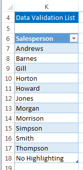
Before we can set up the Conditional Formatting we need to set up the data validation list. So, over in column K I have the list of Salesperson’s names.

I’ve also added an item to the list for ‘No Highlighting’. Since there is no Salesperson called ‘No Highlighting’ it simply won’t display and conditional formatting if you select it.

no highlighting

In cell C4 I’ve got my Data Validation list which references the Salesperson’s names in cells K7:K18:

data validation list

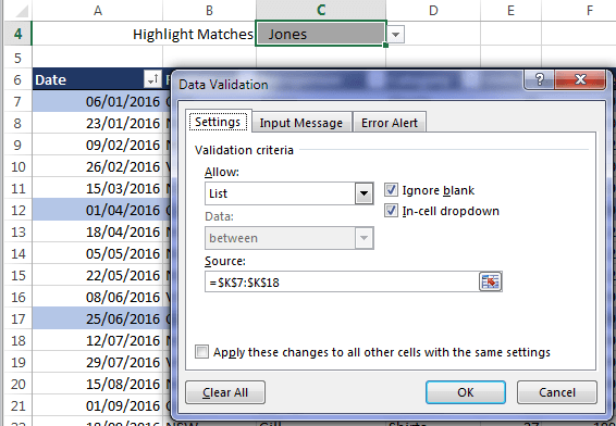
If you don’t know how to insert a Data Validation, or Drop Down list as they’re sometimes known, then click this link to read the tutorial on Data Validation: https://www.myonlinetraininghub.com/excel-drop-down-lists

Setup Conditional Formatting

Now all we need to do is set up the Conditional Formatting to highlight rows that match the salesperson selected in the Data Validation list.

Step 1: Select all of the cells you want the Conditional Formatting to apply to. In my case it’s cells A7:G49.

Step 2: Home tab > Conditional Formatting > New Rule > select ‘Use a formula to determine which cells to format’ from the Rule Type list.

Step 3: Insert the formula =$C$4=$C7:

insert formula

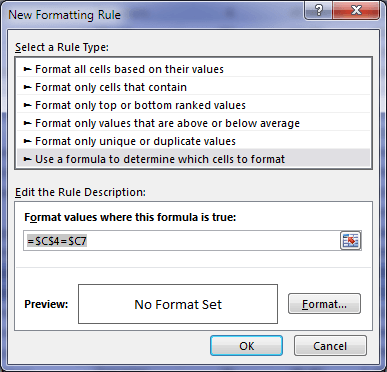
Note: The absolute referencing in this formula is the key to success. Get this wrong and you’ll be scratching your head trying to understand what is going on.

Let me explain:

Conditional Formatting formulas must evaluate to TRUE or FALSE. When the formula evaluates to TRUE the format is applied, and when it evaluates to FALSE the format isn’t applied.

$C$4: We absolute both the column and row reference here because this is the cell containing the Salesperson’s name selected in the Data Validation list and we want that cell tested for every row.

$C7: We reference the first cell in column C of the table, and we only absolute the column reference here because we want the Data Validation formula to move down through each row in column C to check if the salesperson matches the salesperson selected in the Data Validation list in cell C4.

If that’s hurting your head then I recommend you take a few minutes to read my tutorial on how Conditional Formatting formulas work. I think the images in that post will help you visualise what Conditional Formatting is doing in the background. Once you get this there’ll be no stopping you.

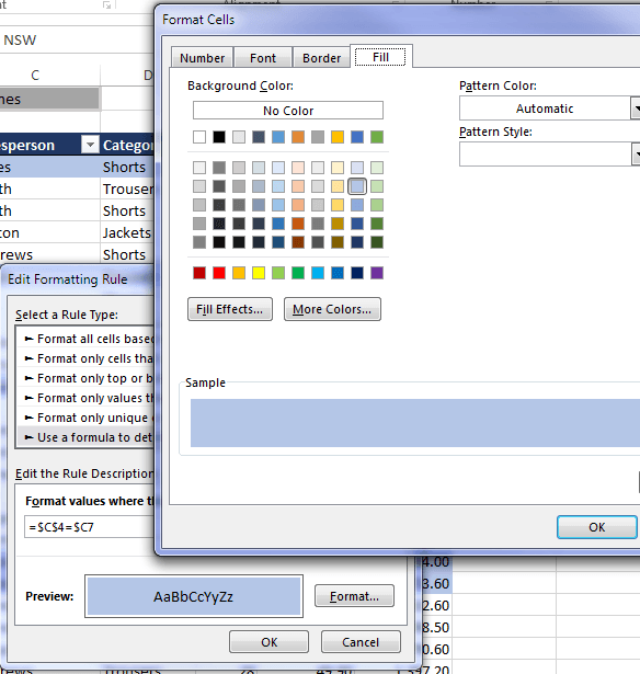
Step 4: Click the ‘Format’ button in the dialog box above and set your format:

set formatting

Job done! The hardest part is getting your head around how to construct the formula.

Excel Conditional Formatting Thumb

More Excel Posts

linear regression

Excel Linear Regression

Excel linear regression is easy with the built-in tools. Use charts to plot linear regression or use the Data Analysis Toolpak.
speed up slow excel files

How to Improve Excel Performance

How to improve Excel performance and the various causes of slow Excel files so you can speed up Excel and avoid problems in future.
Securely Share Excel Files

Securely Share Excel Files

Securely share Excel files stored locally, on OneDrive or SharePoint. Prevent editing or downloading, specify who can open and edit the file.
excel check boxes

Interactive Excel Check Boxes

Excel check boxes are interactive elements you can link to formulas, charts, conditional formatting and more.
tips for working in multiple excel files

Hacks for Working in Multiple Excel Files

Awesome tips for navigating, arranging and working in multiple Excel files. Guaranteed to streamline your workflow and increase productivity.
chatgpt for excel

ChatGPT for Excel

Using ChatGPT for Excel can be hit and miss. Learn the best uses for ChatGPT to make your Excel life easier and what to avoid using it for.
excel templates

Where to Find Free Excel Templates

Where to find free Excel templates and how to create your own Excel templates. Using templates saves time and effort.
Easily Remove Password Protection from Excel Files

Easily Remove Excel Password Protection

How to remove Excel password protection when you’ve forgotten the password. Works for sheets, workbooks and read only files.
Import data from a picture to Excel

Import Data from a Picture to Excel

Import data from a picture to Excel. Works with pictures from a file or the clipboard and loads it to the spreadsheet.
excel online

5 Excel Online Features Better than Desktop

5 Excel Online Features Better than Desktop including searchable data validation, track changes, single line ribbon and more.


Category: Excel
Previous Post:Return an array from a udfReturn An Array From A UDF
Next Post:Excel Custom Number Format Guide

Reader Interactions

Comments

  1. Bobbie

    December 11, 2020 at 2:59 am

    This is amazing! I am wondering though, can the first value be multiple cells? I have a static list of people that I want to highlight a certain color, but I can’t get it to highlight anyone but the first name. I tried $Q$5:$Q$10, but only the name in Q5 highlights. Thanks!

    Reply
    • Mynda Treacy

      December 11, 2020 at 10:07 am

      Hi Bobbie,

      Please post your question on our Excel forum where you can also upload a sample file and we can help you further.

      Mynda

      Reply
  2. EJAZ HUSSAIN

    June 2, 2020 at 12:49 pm

    It is a best website for me as i am facing some problems in excel. So it will help me

    Reply
    • Mynda Treacy

      June 2, 2020 at 7:08 pm

      Glad we can help, Ejaz!

      Reply
  3. Khaled Naser

    February 12, 2017 at 5:26 pm

    Hi Mynda
    Nice article. Is it possible to put data validation in another worksheet if I have a big list?

    Reply
    • Mynda Treacy

      February 12, 2017 at 7:45 pm

      Absolutely. I just put it on the same page for teaching purposes.

      Mynda

      Reply
  4. Shakil

    February 11, 2017 at 5:28 pm

    Awesome

    Reply
    • Mynda Treacy

      February 11, 2017 at 6:55 pm

      Glad you liked it, Shakil 🙂

      Reply
  5. David

    February 11, 2017 at 3:39 am

    Mynda

    I really like this tip. So simple and very impactful.
    I have passed on to others.
    You are the best.
    David

    Reply
    • Mynda Treacy

      February 11, 2017 at 10:46 am

      Cheers, David! Glad you’ll find it useful and thanks for sharing it 🙂

      Reply
  6. Katy Potter

    February 10, 2017 at 4:12 am

    Trying to think of a situation where this would be desired, as opposed to just filtering the column headers to filter to the salesperson you want to locate the data for?

    Reply
    • Mynda Treacy

      February 10, 2017 at 8:34 am

      Hi Kathy,

      If you want to still see the other data for the purpose of comparisons is one scenario I can think of. Also, in big tables filtering on and off can be slow.

      Mynda

      Reply
  7. Renny Schweiger

    February 10, 2017 at 1:40 am

    Fabulous! Also, the How Conditional Formatting Formulas Work tutorial is gold. Thanks for this. I’ve struggled with this at times and this makes it crystal clear.

    One upgrade to this is to make the table (range) a Table, i.e., Format as Table. The drawback of the current conditional formatting is that if you add a row to the bottom of the range the formatting doesn’t automatically apply (unless you copy the formatting). If you convert the range to a table, the conditional formatting now applies to the table (“Show formatting rules for: This Table” in the Conditional Formatting Rules Manager) and any new rows added will automatically get the new formatting.

    Another small improvement is to name the cell with the validation; for example “NameToHighlight”. Then the cond. formatting formula becomes =NameToHighlight=$C7.

    Now if we could only figure out why Excel doesn’t allow us to use table structured references in the conditional formatting formula; If I named my table “TableToFormat” the formula would be =TableToFormat[@Salesperson]=NameToHighlight. So much nicer to read….

    BTW, I love tables now. I bought the book by Barresse and Jones I think because I saw it advertised on your site.

    All the best.

    Reply
    • Mynda Treacy

      February 10, 2017 at 8:35 am

      Great ideas, Renny. Thanks for sharing them and I’m so pleased you’re a Tables fan now 🙂

      I agree it would be great if we could use the Structured References in more places. Maybe Microsoft will fix that some day.

      Mynda

      Reply
  8. Toba

    February 10, 2017 at 1:10 am

    Can this work for the Sort function or a Filter? So the data will only show the cells that are TRUE and filter/ Sort out the rest?

    Reply
    • Mynda Treacy

      February 10, 2017 at 10:42 am

      Hi Toba,

      I’m not sure I understand the scenario. You could add a column to your data set that tests if a value/row meets a condition and return a TRUE or FALSE which you could then use for sorting or filtering. You’d need to write some VBA code to automate that though, otherwise you’d have to change the sort/filter manually.

      Mynda

      Reply
  9. Jim Hundertmark

    February 9, 2017 at 11:42 pm

    I found this tool to be extremely useful at finding pieces of data within large data sets quickly. Is there a way to have the data validation list auto-populate with the unique values within a column? Thus, instead of having a separate list, the data validation looks at the column and auto-populates all the names.

    Reply
    • Catalin Bombea

      February 11, 2017 at 3:28 pm

      Hi Jim,
      There are many solutions for data validation lists, that can remove the blanks from a column, or list the unique entries only. Please take a look at this article, a solution based on a pivot table might be the solution you need.
      Catalin

      Reply
  10. Peter Buyze

    February 9, 2017 at 10:17 pm

    Mynda, this tutorial is a little gem, as all your tutorials are.
    Correct me if I am wrong but what you show here is a different way of filtering, isn’t it?
    And if so, isn’t it just as easy to use the filter arrow in cell C6?

    Reply
    • Mynda Treacy

      February 10, 2017 at 8:38 am

      Hi Peter,

      Thanks for your kind words 🙂

      This doesn’t filter as such so you can still see the highlighted rows in the context of the whole data set. Maybe you want to still be able to see the other rows for reference, whereas with the Filter buttons you only see the selected data.

      Horses for courses.

      Kind regards,

      Mynda

      Reply

Leave a Reply Cancel reply

Your email address will not be published. Required fields are marked *

Current ye@r *

Leave this field empty

Sidebar

More results...

launch excel macros course excel vba course

Featured Content

  • 10 Common Excel Mistakes to Avoid
  • Top Excel Functions for Data Analysts
  • Secrets to Building Excel Dashboards in Less Than 15 Minutes
  • Pro Excel Formula Writing Tips
  • Hidden Excel Double-Click Shortcuts
  • Top 10 Intermediate Excel Functions
  • 5 Pro Excel Dashboard Design Tips
  • 5 Excel SUM Function Tricks
  • 239 Excel Keyboard Shortcuts

100 Excel Tips and Tricks eBook

Download Free Tips & Tricks

Subscribe to Our Newsletter

Receive weekly tutorials on Excel, Power Query, Power Pivot, Power BI and More.

We respect your email privacy

239 Excel Keyboard Shortcuts

Download Free PDF

mynda treacy microsoft mvpHi, I'm Mynda Treacy and I run MOTH with my husband, Phil. Through our blog, webinars, YouTube channel and courses we hope we can help you learn Excel, Power Pivot and DAX, Power Query, Power BI, and Excel Dashboards.

Blog Categories

  • Excel
  • Excel Charts
  • Excel Dashboard
  • Excel Formulas
  • Excel PivotTables
  • Excel Shortcuts
  • Excel VBA
  • General Tips
  • Online Training
  • Outlook
  • Power Apps
  • Power Automate
  • Power BI
  • Power Pivot
  • Power Query
microsoft mvp logo
trustpilot excellent rating
Secured by Sucuri Badge
MyOnlineTrainingHub on YouTube Mynda Treacy on Linked In Mynda Treacy on Instagram Mynda Treacy on Twitter Mynda Treacy on Pinterest MyOnlineTrainingHub on Facebook
 

Company

  • About My Online Training Hub
  • Disclosure Statement
  • Frequently Asked Questions
  • Guarantee
  • Privacy Policy
  • Terms & Conditions
  • Testimonials
  • Become an Affiliate

Support

  • Contact
  • Forum
  • Helpdesk – For Technical Issues

Copyright © 2023 · My Online Training Hub · All Rights Reserved. Microsoft and the Microsoft Office logo are trademarks or registered trademarks of Microsoft Corporation in the United States and/or other countries. Product names, logos, brands, and other trademarks featured or referred to within this website are the property of their respective trademark holders.

Download A Free Copy of 100 Excel Tips & Tricks

excel tips and tricks ebook

We respect your privacy. We won’t spam you.

x