Excel’s Conditional Formatting tool is diverse with loads of built in rules that you simply point and click to use, but I find more often than not that I need to use a formula based rule.
I can sympathise if you’ve ever tried to use formulas in your conditional formatting and ended up tearing your hair out in frustration.
Thankfully there are only 3 simple rules you need to know. Once you understand these rules you’ll never look back.
Watch the Video

Conditional Formatting with Formulas - Written Instructions
Rule 1 – the formula must evaluate to TRUE or FALSE*
Conditional formatting is looking for a true or false outcome, or their numeric equivalents 1 and 0. If the outcome is true or 1 it will apply the format, if it’s false or 0 it won’t. It’s black and white.
*A little known fact is formulas that evaluate to any positive or negative number will also be considered as 'TRUE' and the format will be applied. And any formulas that evaluate to zero will not have the formatting applied.
I like to test my rules in the worksheet first. Once I know they’re returning the correct result I can create my new rule and paste the formula into the conditional format rule description.
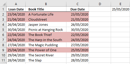
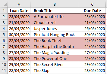
For example, let’s say we have loaned out some books and we want to flag when they are overdue by formatting them in red like this (by the way, my dates are formatted dd/mm/yyyy):
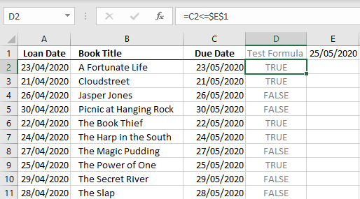
In cell E1 I have the current date, and in column D I’ll enter my test formula:
=C2<=$E$1
Then I can copy the formula down the column and check each row is evaluating as I’d expect.
Ok, now I’m happy with my formula I’ll edit cell D2 and copy the formula to my clipboard so it’s ready to paste into the Conditional Formatting rule description.
Rule 2 – Select Your Cells
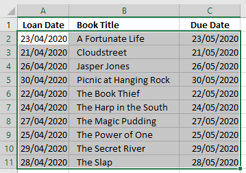
Before you go and set up your conditional formatting rule you need to select all of the cells you want formatted.
Since I want to format from column A to C for each row, I’ll select my whole table like this:
Rule 3 – Absolute References
The next trick with Conditional Formatting formulas is when to use absolute references.
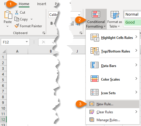
I’ll create my new rule:
And paste my formula into the 'Format values where this formula is true' field:
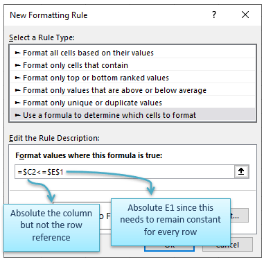
As I’m comparing the dates in column C to our current date, I need to absolute the column reference in my formula, but not the row reference.
And that’s because in the background Excel is applying that formula to every cell I selected (back in rule # 2) to test for a TRUE/FALSE outcome.
This is the way I remember this rule:
When you enter the formula in the 'Format values where this formula is true' field Excel is applying it to every cell you have selected.
When it does so, the cell references dynamically update, just as they would if you entered it in cell C2 and then copied and pasted it over your selected area, except instead of actually pasting it the Conditional Formatting tool does the calculation in the background.
I picture it as a separate layer of the workbook, like in the image below. The top layer is the Conditional Formatting formula and the bottom layer is my workbook.
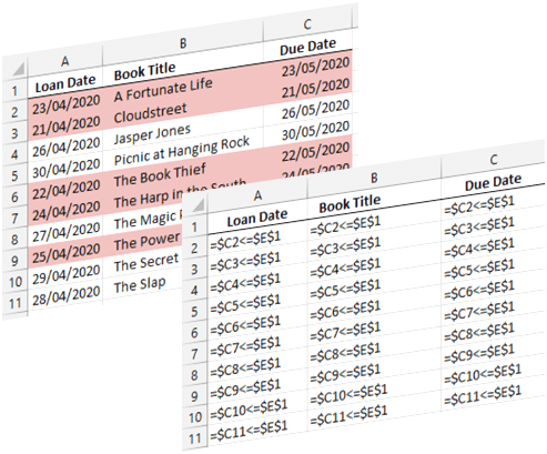
Note how in the Conditional Formatting layer the formula in each row has dynamically updated to pick up the current row but the column reference remains with C. i.e. testing the due date in column C for each row.
It would then evaluate like this:
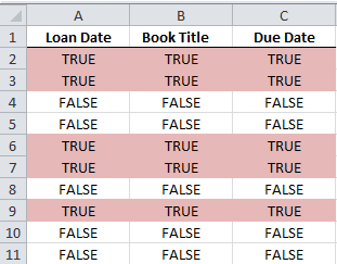
If I didn’t absolute column C Excel would think I wanted to do this:
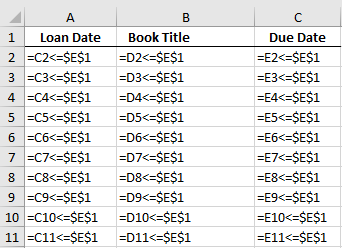
See how the above formulas would be wrong since it’s testing every cell to see if it’s < or = to cell E1 not just column C for each row?
Ok, now that I’ve entered my formula I can set up my formatting and I’m done:

Hi Mynda,
I have a table with almost 20 different conditional formatting rules per line.
I want to extrapolate the conditional formatting so that I dont have to adjust it line by line for every cell.
Is there an easy way to do this?
Hi Elmarie,
Other than with VBA, you have to edit each rule and change the ‘applies to’ range to include multiple cells.
Mynda
Hi I am trying to format certain cells in a work book using dates and the sum of 2 colums as the criteria. I have a list of customers in col A, settlement date in col B, deposit $ in col c, deposit $ returned in col D. At certain points in time I need to refund deposits. What I would like to achieve is if today’s date is settlement date + 15 days and Col C-Col D is not $0 format col C in red
Hi Janey,
Try this formula:
Mynda
Hi Mynda, thanks for the above info. I now want to change the formula slightly so instead of Col C& D being numbers, I want the a cell to format if Col D is today +15 days & col f is blank
Hi Jane,
Mynda
Hello, I have been trying unsuccessfully to create a conditional format. Here is what I would like to accomplish:
I want the values in columns BJ and BL to be in red, as a result of two conditions: if the value in BM is greater or less than 0, AND if BO is blank.
I tried this formula, but it came back as an error:
=AND ($BM20, $BO=””)
Any help would be greatly appreciated!
Hi Warren,
Try this one, applied to rangeBJ2:BJ1000:
=AND($BM2<>0, LEN($BO2)=0)
(the row number from formula should match the row number from the applied range)
I would like to know if we can apply conditional formatting to a cell if that cell’s value is changed?
Hi NY,
No, not with Conditional Formatting, only with VBA.
Mynda
Thanks for the reply. Are you able to help with the code in VBA?
Please post your question in our Excel forum.
I avoid using conditional formatting but after reading your article, it looks easy.
Your explanation of the concepts is superb. Well Done!
Thanks, Farooq. Glad you’re keen to give it a go 🙂
Mynda
I’m trying to format a cell to be highlighted when it is < 89% of another cell
B2 50 and D2 100
I want B2 to color red if less than 89% of D2, and if B2 is 90%-99% of D2 yellow, and if B2 is <=100% of D2 green
Is this possible?
Hi Leah,
Yes, it’s possible. You’ll need a separate format for each colour. Set them up in the order below, that way the yellow rule will override the red rule and the green rule will override the yellow and red rules.
Red: =$B2/$D2<89%
Yellow: =$B2/$D2>89%
Green: =$B2/$D2>=100%
Select all of the cells you want to apply the format to before inserting the formats.
If you get stuck please post your question and sample Excel file on our Excel forum.
Mynda
Hi,
I have list with data from two sources.
It takes figures for each month in the year.
One source takes place in odd rows and the other in even rows and I want to highlight cells that do not match (both sources should be identical).
The way I do it is to conditional formatting one cell (no absolute) like b3b2, copy it to the entire row and then copy it (with the brash) to each other row.
I can write a macro to do the job but wonder if there is a way to do it with the conditional tools only.
Hi Alex,
There is no tool that I know to apply the format to other rows in mass, only workarounds as you mentioned.
I’m trying to setup a formula for the following:
Column Q is tracking expiration dates (for permits). Column W is tracking updated expiration dates.
Column Q already has conditional formatting to fill RED when the date is expired. I’d like Column Q to format back to “no fill” if there is a date entered into Column W.
Does that make sense, and is it possible to do?
Hi Keri,
Yes, just add another rule to test if column W contains a value. This will override the first rule.
Mynda
Very Helpful post, this will make my formatting more useful to identify cells that meet specific date criteria.
Much Appreciated
Thanks, Adrian. Glad you’ll find a use for it.
Mynda
Many thanks Mynda. I Have tried to explain conditional formatting to my accounting staff, but was never able to create a visual that’s unforgettable–as you provided above with the “layering”
Fantastic, Gordon! I’m so pleased you found it useful. It was something that I struggled with in the beginning too.
Cheers,
Mynda
Mynda, I think I just figured it out. Needed to change my formula to be AP63=TRUE and have it change the font to black from white. This seems to work. Don’t understand why the opposite scenario didn’t work – but at least this works now!
Thanks for your great tips!
Glad you figured it out, CJ 🙂
I have a Check Box linked to cell AP63. When the Check Box is unchecked (making cell AP63 contain “FALSE”), I would like range C89:Y98 to change font color from black to white. Is this possible? I thought I could get it to work with Conditional Formatting, but it doesn’t seem to be working for me. I use a formula in Conditional Formatting of: =$AP$63=FALSE. Then I set the font color to be white. It doesn’t work – any ideas?
Hi there – I have really enjoyed your webinars and our Customer Service Analyst purchased your Excel for Customer Service Professionals course back in July. She is getting a lot of mileage from it. One thing I am having trouble with and I cannot find any good examples online, is the following: I have a simple spreadsheet tracking issues including date resolved and current status. I am using the built-in conditional formatting rules for “Highlight Date occurring.” So that last week, last month and yesterday and today are red. Tomorrow, next week and next month are green. I also have as the first condition, no format set. Basically I would like to clear all formatting if the current status column has “Completed.” I have tried different combinations of formulas including IF AND statements combined with TODAY() and I cannot get this to work! Help a poor soul dying a slow death by Excel in Texas????
Hi Gina,
Great to hear your analyst is enjoying the customer Service course 🙂
We’d be happy to help you with your Conditional Formatting conundrum. Can you please post your question and workbook (or sample workbook) on our Excel Forum so we can see your question in context and give you a specific answer.
Thanks,
Mynda
Hi,
Let’s say I have a Target number and an Actual number, if the Actual number is grater than the Target one I need the cell to be green. If the Actual is less, I need the cell to be red. I have done this using the less than and greater than rule.
However, now I need the Actual cell to be yellow if it is less than 3% below the Target number. I am not able to get this part to work. Any advice?
Hi Dayan,
You can use this formula:
=Actual/Target>=0.97
Mynda
regarding above ex..in column if it is amounts. how to add that paricular amounts(total amounts) in cell f.
Hi Jerald,
Try this formula:
Catalin
I ran across a conditional format that I can figure out the formula says:
=ActualBeyond
or
=plan
But there are no named ranges and i cannot find any links to these. how is this done… Any thoughts?
Hi Mark,
I suspect these names are referencing UDF’s (User Defined Functions). Check in the VB Editor for them.
Kind regards,
Mynda
Hi. I have a column of dates. I would like to see which dates are within 30 days from today and have it filled in color red.
The conditioning formula I used is =B7-TTODAY()<30. But why is it that dates like feb, march, may are also filledmin red?
Hi Che,
I suspect there is something wrong with the format of the date in cell B7. Assuming your formula is actually
If you’d like to send us your file via the help desk we can troubleshoot what might be the problem.
Mynda
Just sensational tutorials, many thanks
Kind regards
maggie
Wow, thanks Maggie 🙂 Glad we could help.
BOX/SKID? FULL LAYERS
box 58
box 61
skid 12
box 20
skid 15
If it is a box, I need to know if the full layers are over 60 so I can calculate a new skid and if it is a skid I need to know if it is over 12 layers, I need to calculate a new skid
So my question is this: is there a conditional formatting I can use that will highlight any boxes that are over 60 and any skids that are over 12? They do share the same columns.
Thanks so much
Amy
Use conditional formatting with these formulas:
=AND($A2=”skid”,$B2>12)
=AND($A2=”box”,$B2>60)
The range of values are assumed to start from row 2.
Cheers,
Catalin
Thanks. I have added these rules, but one small issue. It is highlight two cells above the one it should be? The cells are not next to one another, would that cause an issue? Cells are “Y” and “AB”
Thanks
Amy
Hi Amy,
I have to see what you have done, hard to tell… The range to highlight must be correlated to the formula: for example, if the range starts from AB2, the formula should refer to the same row, row 2: IF($Y2=”box”……, and the second check should start from the same row 2: IF(AB2>60….
Can you upload a sample workbook on Help Desk? https://www.myonlinetraininghub.com/helpdesk/
I will gladly help you 🙂
Cheers,
Catalin
Oh, I see. I had selected the range starting at Y1, not Y3, so I corrected and now it is fine. Awesome. Thanks so much for your help. You guys are amazing!!!
Amy
Glad it works fine for you Amy, you’re always wellcome.
Catalin
Great explanation. Just curious, rather than entering a date in E4, could the cell be formatted to default to the system date?
Hi Mary,
You are right, you can enter a formula to return system date: =TODAY() or =NOW()
Cheers,
Catalin
I’m trying to make a formula that changes the coloring of different rows to make them color coded by the difference of the date that is in the cell and the current date. This is items that we need people to give us paperwork for annually, and the dates in the cells are the dates we have for the item. If the item is overdue (todays date a year ago or earlier) I want it to be the standard “bad” cell style (light red with dark red font) if it is within one month of being overdue I would like it to be the standard neutral style (yellow and yellow) and if it has more than 1 month to be overdue I would like it to be the standard good style (green and green.) I can put in the colors myself if someone can tell me how to do the formula. Thanks!
Hi Ashley,
This formula will tell you if the date in cell E8 is more than a year ago:
The TODAY function returns the current date as per your computer clock. All you need to do is calculate what the date would be for each of your criteria and then compare that date to the dates you have to see if they are less than or greater than your calculated date.
I hope that helps put you on the right track. Please let me know if you get stuck.
Kind regards,
Mynda.
Hello, I am trying to create a conditional formatting sheet which shows either ‘yellow’ when today’s date is within 2 months of a set date and ‘red’ when today’s date is within 1 month of today’s date.
Basically, I have a spreadsheet with a list of dates of certificates and when they expire. What I want to be able to do is to have excel highlight the cell when it is going to expire both 1 month and 2 months away so that I can look at my spreadsheet and see visually when I need to remind people to renew their certificates.
I have tried so many ways and I feel so stupid because I just cannot get it to work. All other examples I have found make the colour change AFTER today’s date and not before.
HELP
Hi Israel,
You can use this formula for dates <60 days from today:
=B2-TODAY()<60
Where B2 is your 'set date'.
And for <30 days you can use this:
=B2-TODAY()<30
I hope that helps.
Kind regards,
Mynda.
I have a quick question. Currently I have a spreadsheet that is grouped up by columns. Meaning I have a total of 20 columns but they are broken into sub groups. The 1st group contains 10 columns, the 2nd group contains 6 columns and the 3rd group contains 4 columns. Ultimately what I would like to do is everytime the 1st group edits the row for the entire row to shade yellow. Anytime the 2nd group edits that row for the entire row to shade amber and finally anytime the 3rd group edits the row for the entire row to shade say light blue. Esentially my goal is that anytime a group edits the row whenever someone goes back into the spreadsheet that person will know who made the changes. Is this possible?
Hi Shekhar,
What happens is they don’t edit it in order? Excel can’t tell who edited it last. You could have a rule that shaded the row the specific colour based on which group had data in it, but if they don’t edit the row in order (group 1 first, group 2 second and group 3 third), it won’t work.
A slightly different solution would be to have a drop down list that the person editing selected their name from before saving the file. This way the next person to open the file would see who was in it last.
If you wanted to automate this you could do so but it would require VBA.
Kind regards,
Mynda.
I think that we help me
Glad to help, Ilias 🙂
I have a spreadsheet where employees daily record defects in equipment. They use data validation (drop down box) to record common defects or select No Defects if everything is fine. I want yellow fill to be applied whenever a defect is noted. If No Defect is noted (or if the cell is blank) I want no fill applied. I can use conditional formatting to apply no fill when No Defects is entered, but then the rest of the spreadsheet (or cells selected) is always yellow. I want no fill unless a defect is specified. Can I do this?
Hi Vic,
Yes, conditional formatting can do that.
It sounds like you have the whole worksheet highlighted yellow and you remove the formatting with the conditional formatting. I would do it the other way around.
If you get stuck feel free to send me your workbook via the help desk. Please repeat your instructions so I can easily help you.
Kind regards,
Mynda.
thanks
You’re welcome, Dante 🙂
Thank you for this sharing.
You’re welcome, Ravi 🙂
Hi. How do you apply conditional formatting in reverse?
Per definition: Conditional formatting is applied to one or more cells and, when the data in those cells meet the condition or conditions specified, the chosen formats are applied.
How can I rather apply a certain condition to a cell with a chosen format? For instance: some cells in a pricelist contain green highlighted prices. Those prices should be treated different from the rest. I want a way to test “format of the cell is green” as a TRUE or FALSE.
Hi Adri,
You need VBA to do that. There aren’t any formulas that can detect cell colour.
The only other option is to apply filters to your data and manually filter on the cell colour.
Kind regards,
Mynda.
Thanks Mynda for your answer. You potentially saved me many frustrating hours of searching for nothing 🙂
I personally do not like filters at all, it feels like a copout for writing proper formulas!! That is why I started looking for a formula based solution. I never know what happens to cells between the filtered cells when I copy or paste or add comments etc. But I guess filters is the middle way until I learn how to use VBA.
I understand your concerns with the filtered cells. Some things skip them and others don’t. From memory pasting comments seems to be applied to all cells hidden or not.
1. Go Insert>Name>Define and name this formula that you are about to create “color”
2. In the Refers To box type:
=GET.CELL(63,OFFSET(INDIRECT(“RC”,FALSE),-1,0))
3.Back in the sheet, in the immediately adjacent cell below the one where you want to determine the fill colour type (so yellow cell in A1, then you enter the following in A2):
=color
This will return the colorindex of the cell interior (6 is bright yellow in a default installation).
So you can use this in a formula to do as you wish eg:
=IF(color=6,1,”It ain’t yellow”)
Thanks for sharing, Riaan.
Note: GET.CELL is an old XLM4 Macro function (VBA) with very limited use.
Hi!
“Excel conditional formatting row color” are used commonly in data entry task or managing data. So thank for sharing this important information.
I have find out some other links that’s also helpful for beginner.
Thanks for sharing, Alex 🙂
I recently started reading your articles on excel and formulas Mynda. I have to say you go in depth with great illustrations which makes it so much easy to understand for readers. Thank you, since I learned alot and will use some of your techniques on my articles. Keep up the good work!
Hi Tobi,
On Behalf of Mynda,
Thank You!
Cheers.
CarloE
Hi Mynda and Carlo,
I have 26 Columns, the first 9 are white coloured cells to imput data. The other remaining columns are coloured gray to remind me not to touch them as they have formulas in them to automatically fill in when I put data into the first 9 columns.
Within the first 9 columns I have two with dates in them, one has an entry date (column 4) and one has an exit date (column 7).
What I would like to achieve is when these 9 columns/cells are empty they remain white, as they are now.
When I input an entry date (column 4) into the cell I would like these first 9 columns/cells to be filled with the colour yellow. But once I put in the exit date (column 7) I would like these first 9 columns/cells to be filled with the colour gray matching the other 17 columns/cells to distinguish that this row is finished with.
Any help would be appreciated, I can get a few things going ok but not the lot at once. Many thanks.
Kind Regards …. Max
Hi Mynda & Carlo,
I have worked this out eventually, I hope you haven’t spent any time on it as of yet.
Many thanks all the same.
Cheers … Max
Good that you figured it out already. CHeers Max!
Hi Carlo & Mynda,
Well … I thought I had it worked out.
I got 1 row working so thought I’d be able to expand the ‘applies to’ area and it would be all done, simple but no, something is wrong.
I have 1500 rows within this sharetrading spreadsheet.
If you can take a look at this for me that would be fantastic.
Many thanks again …. Max
HI Carlo & Mynda,
Well after some time finally got it finished.
Thanks for all the tips and clues on the website, it steered me in the right direction to get this done.
Respect your efforts to help others, very generous.
Kind regards … Max
Cheers Max on Behalf of Mynda! 🙂
As always, I would like to thank you for your great explanation on how to work on Excel in a simple and visual way.
Thanks, Weynshet 🙂
I have a series of time in one column and a series of time in another column. Each column represents a different process. I want to assess each row for the two time columns and conditionally format the times in one column that are greater than the times in another column.
1…..00:22:06……….00:26:36 – since the second column with time is greater than the first column, I’d like to format the second column in a color to make it stand out.
Mary
Hi Mary,
1 Go to Home Ribbon
2 Click Conditional Formatting
3 Add Manage Rules
4 CLick New Rule
5 Select Rule Type: Use Formula to determine which cell to format
FIRST RULE:
SECOND RULE
Do the same for the second Rule…but this time:
Read more : Conditional Formatting
Cheers.
CarloE