PivotTables are the Origamists of Excel. Folding and summarising data into almost any shape. I say 'almost' because until Excel 2013 they couldn’t calculate a unique (sometimes called distinct) count.
For example, you might want to count the number of 'things' you had, whether it be products or customers, or any other unique combination of records you might want to count.
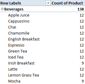
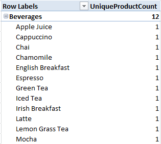
In the example below we can see the count for each product, but this is actually the count of the number of records for each product, as opposed to the number of unique products.
Bummer. You'd think something so simple would be available. Not to worry. Let's take a look at 3 different ways we can count unique items in a PivotTable.
The idea being that you'll find a solution that works with the version of Excel you use.
1. Excel PivotTable Count Unique Items pre 2013
Pre Excel 2013 you need to use a workaround, which is this:
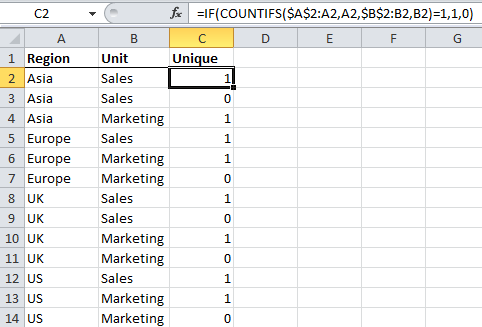
- Add a helper column to your raw data with a formula that counts a 1 for the first instance of the product, and a zero for any duplicates.
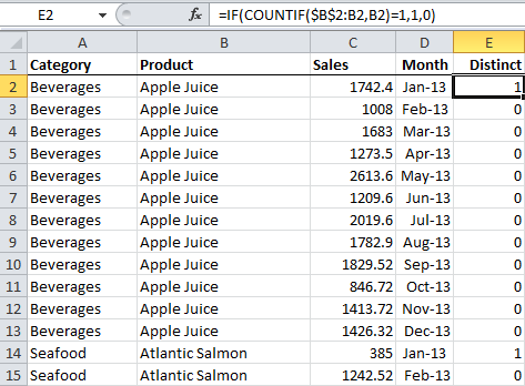
In cell E2 I entered this formula:
=IF(COUNTIF($B$2:B2,B2)=1,1,0)
Then copied it down the column.
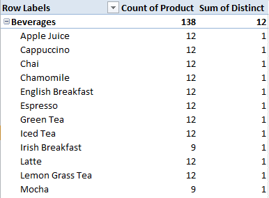
Now I can include a sum of my new ‘Distinct’ column in my PivotTable like this:
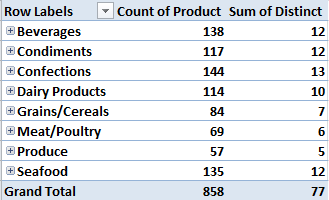
And below I further summarised the Products into their Categories which shows that I have 77 unique products, with the highest number being in the Confections category:
Remember the 'Count of Product' is actually the count of records (in this case they're sales) for each product.
If you had multiple fields you wanted to combine to count unique combinations you could use the COUNTIFS function. As in the example below where I want to count unique combinations of the Region and Business Unit.
Or if you have Excel 2003 you could use a SUMPRODUCT function like this:
=IF(SUMPRODUCT(($A$2:A2=A2)*($B$2:B2=B2))>1,0,1)
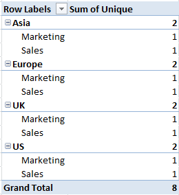
You could then sum your unique Region/Business Unit combinations like this:
2. Excel 2010 PowerPivot Distinct Count
If you’ve got the free Excel 2010 PowerPivot addin installed you can go ahead and try this method.
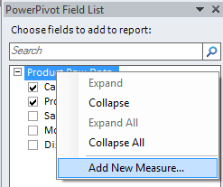
- Insert a PivotTable from within PowerPivot.
- Right click on the table name in the PowerPivot Field list and select ‘Add New Measure…’.

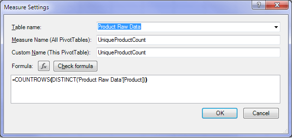
- Give your Measure a name (this is the field name that will appear in your PowerPivot field list).
- Enter your formula =COUNTROWS(DISTINCT('Product Raw Data'[Product]))
Voila, you have a unique count of your products:
3. Excel 2013 PivotTable Distinct Count
What Do You Think?
Did you like this? Let me know by sharing it using the social media icons below, or leave a comment.

I’m trying to set up a pivot table with a distinct count, and then the percent of column total. I use distinct count a LOT! The problem is the percents don’t add up to 100% (even though that is what you see at the bottom of the pivot table. Is there a way to get percents of distinct counts? Why doesn’t it work?
Thanks!
Cheryl
Hi Cheryl,
You’ll most likely need Power Pivot for this type of calculation. Please post your question and sample Excel file on our Excel Forum where we can help you further.
Mynda
Thank you, it worked a treat.
Great. Glad I could help.
It was insightful
Thank you so much for your Excel-lent posts and Webinars.
You’re welcome 🙂
Thanks a lot for sharing such useful information. Its Great
You’re welcome 🙂 Glad we can help.
your site is very rich . i have learnt so much.
Thanks! Glad you’ve found it useful, Dan 🙂
Thanks so much for this info. Tip #1 was just what I needed to solve a pivot table challenge. I had created one to count # of clients seen each month, but also wanted a column to show # days worked. (My detail sheet had duplicate dates for seeing multiple clients in a day). Adding the helper column with your formula worked like a charm.
You’re my hero, as always.
Aw, thanks Wendy 🙂
Glad we could help.
Mynda
I am using the first solution from this article (=IF(COUNTIF($B$2:B2,B2)=1,1,0)) and it works like a charm. The problem is that my spreadsheet has the data refreshed as often as the user would like (they can do it daily or even several times a day) and I have VBA to add the formula and update the associated pivot tables to refresh the report. There are over 24,000 lines of data I am copying this formula to and it is taking a very long time for Excel to process…close to 10 minutes. Is there any way to speed this up?
Hi Lorri,
Depends on what your vba code does…
If you apply the formula with vba in a loop like:
For i=2 to 24000Range("A" & i).Formula="=..."
Next
This will take a lot of time, even if screen updating is turned off.
But if you apply the formula with vba to the entire range like:
Range("A1:A24000").Formula="=...", this is much faster.If you need further help, a sample file will be needed, with your code. You can use our Help Desk if this doesn’t solve your problem.
Cheers,
Catalin
Hi guys. First of all thanks for your attention. Easy question
I’m using this syntax in excel power pivot table
=DISTINCT(ALL(Table2[sedi]) to get as result all the unique values that the field “sedi” displays, despite filters applied in the corresponding pivot table
But i got as result “The DISTINCT function expects a column reference expression for argument ‘1’, but a table expression was used.”
Any tips???
thnx
Dave
Hi Dave,
The DISTINCT function returns a single column table that contains unique values from the specified column. But, DISTINCT can’t return values into a cell or column on a worksheet – you nest the DISTINCT function within another formula, to get a list of distinct values that can then be counted, summed, or used for other operations.
So in this case you’d need to do something like this :
=COUNTROWS(DISTINCT(ALL(Table2[sedi])))
With regards to the specific error you received, sedi must be a column.
Regards
Phil
PowerPivot for Excel can be installed on a computer that has 32-bit or 64-bit Excel 2010. If you have installed the 32-bit version of Excel, you must install the 32-bit version of PowerPivot for Excel. Likewise, if you have installed the 64-bit version of Excel, you must install the 64-bit version of PowerPivot for Excel.
Hi Mynda,
Thanks for posting this, it helped me complete a key part of a project at work today! I was able to reference your “IF(COUNTIF($B$2:B2,B2)=1,1,0)” seen in Option #1 in order to get a Distinct Count column in the data set I was working with.
For whatever its worth, larger data sets similar to mine may have trouble looping through the “$B$2:B2” portion of the statement above. The formula I created (edited to match your Beverages, Apple Juice, etc data set in Option 1 above) is “=IF(AND(A2=A1, B2=B1), 0, 1)”.
NOTE: A key first step before using this “=IF(AND(A2=A1, B2=B1), 0, 1)” formula is to sort both Column A and Column B from A-Z (alphabetical order). This formula can then be placed in cell E2 and copied down the column. This formula compares the value in both column A and B for a particular row to the row directly above it, which is why sorting A-Z is so important.
Feel free to pass this formula along to others in future training.
Thanks again Mynda, wouldn’t have been to work through this as easily if it wasn’t for you sharing your knowledge here!
Rob
Good points, Rob. Thanks for sharing 🙂
Hi, I am a little confused on how this works.
I have a data set on students and I want a unique count of students in a year. I tried your method with the countif formula and then I also used the ‘remove duplicates’ sub tab under the data tab (excel 2010). Both gave me different results. Using the formula gave me a lower count as compared to the ‘remove duplicates’. Why?
I checked the latter and found no duplicates and so my confusion.
Hi FS,
I’m not sure why you’d get different answers. Are you able to send me the file so I can try to understand what is going on.
Thanks,
Mynda.
Fantastic. These tips are the perfect learning tool.
Specific, clearly explained, and not too-much-at-once, they are a perfect way to increase my Excel skill level.
Thankyou Mynda
Wow, thanks, Rachael 🙂
Valuable article indeed! The no. of times I have been bemused with the weird nos. in pivot is countless. Thanks for highlighting the problem and solution. I use excel 2010, so the powerpivot setting should help. Though my computer refuses to let me instal powerpivot add in.. Don’t know what the issue is… Any idea what the reason could be.
Thanks,
Hi AS,
Try this one:
If you do not see the PowerPivot tab after you install Office 2010 and PowerPivot for Excel, try the following:

    Load the add-in by clicking File, Options, and then Add-ins. In the Add-ins area, click Manage, select COM Add-ins, and click Go. In the COM Add-ins window, select the Microsoft.AnalysisService.Modeler.FieldList.Addin.Integration check box and click OK.

    If the add-in does not appear after you completed the above steps, and you are running Windows XP and do not have SP3 installed. You will need to install SP3 in order to use PowerPivot. You can download SP3 from the following location: https://www.microsoft.com/downloads/details.aspx?displaylang=en&FamilyID=68c48dad-bc34-40be-8d85-6bb4f56f5110

    If the add-in still does not appear and you installed Excel 2010 and PowerPivot only, you will need to install Office Shared Tools also. With the Office Beta, VSTO is installed when Office Shared Tools is installed. If this is the situation that you are encountering, you need to uninstall PowerPivot for Excel and Excel 2010. Next, install Excel 2010 and Office Shared Tools, and then install PowerPivot for Excel.
Cheers.
CarloE