Excel Dependent Data Validation

I’ve written about how to create dependent data validation lists before here; Excel Data Validation with dependent lists, and here; Dynamic Dependent Data Validation. However the approach I’m going to cover in this tutorial is probably the best I’ve seen, especially if you have a lot of dependencies as it’s easily scalable.

What is Dependent Data Validation

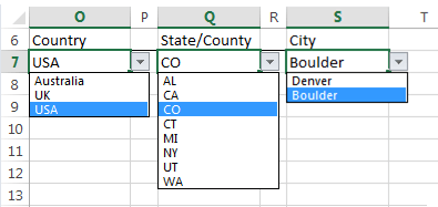
Dependent data validation is where you have a series of data validation lists that display a different list dependent on the selection chosen in the preceding list.

In the image below you can see when the USA is selected in the first data validation list, the state validation list only displays US states. And with CO selected in the State data validation list, the City validation list only displays cities in Colorado.

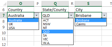
If I select a different country, the state and city lists dynamically update to display related items:

Note: If you choose a different country/state the cells containing the data validation lists (Q7 and S7) don’t re-set, but you could write some VBA code to clear them out if a different country/state was selected.

Download Workbook

This tutorial has quite a few moving parts so it will be easier to follow along if you download the workbook and reference it as you read the steps below.

Note: for the purpose of this tutorial the source data, PivotTables and data validation lists are all on the same sheet so you can see them side by side, but in practice it’s best to keep your workings (source data and PivotTables on separate sheets to your data validation lists).

 

Excel Dependent Data Validation Setup

There are a few steps to set up dependent data validation lists so let’s take a look at the process.

1.      Source Data

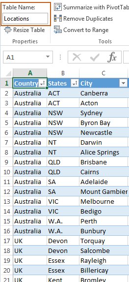
We start with a list of our countries, states and cities formatted in an Excel Table (mine is called Locations):

Of course you might have products, projects, or other hierarchical data.

Count Column

We need to add a column that counts the number of states and apportions 1 across each record so that when you add up the count for a particular state it adds up to 1. What??? I’ll show you what I mean.

In the image below we can see the COUNTIF formula in column D. In column B (State) ACT has two records with each count in column D resulting in 0.50, so the total of ACT’s count equals 1. Likewise, NSW has three records and each count is .333’ so when added up we get 1.

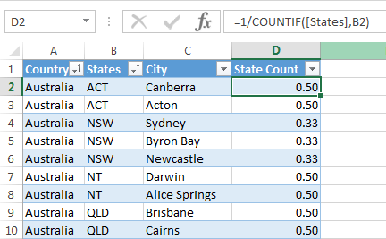
Let’s understand the COUNTIF formula in cell D2:

=1/COUNTIF([States],B2)

In English the COUNTIF part of the formula reads: COUNT the states in the ‘States’ column IF they match the value in B2, which is ACT.

We then divide 1 by the COUNTIFS result to apportion 1 over the rows for that state. We use this column in a PivotTable to find out how many states we have for each country.

2.      PivotTables

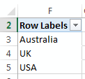
Next we create 3 PivotTables; one for the list of countries:

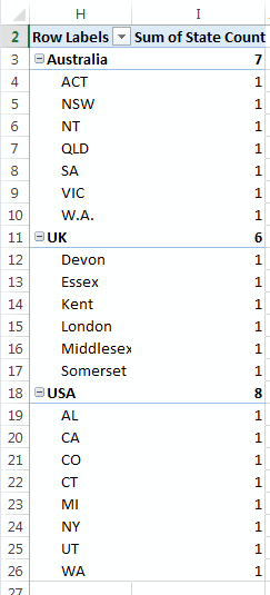
One for the list of states and state count we created with the COUNTIF formula:

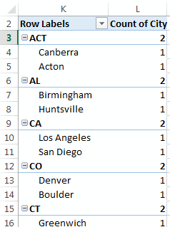
And one for the list of cities and city count:

We use these PivotTables as the source for our data validation lists. And the nice thing about using PivotTables is if the source data changes we just Refresh All (Data Tab) and everything is updated.

Tip: remove the Grand Totals from the PivotTable as they’ll interfere with the next step.

3.      Dynamic Named Ranges

We use three dynamic named ranges  (country, state and city) to find the relevant section of the PivotTables that we want displayed in each data validation list.

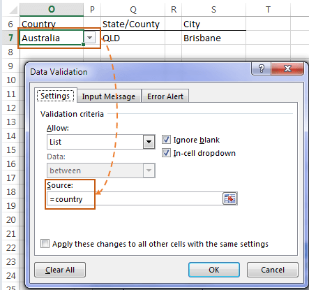
For example, in the image below we can see the Country data validation list source is a (dynamic) named range called ‘country’:

I’ve used the OFFSET Function to create the dynamic named ranges. I won’t go into great detail on how OFFSET works, you can learn it at the above link, but I’ll do a quick recap.

OFFSET Function

The OFFSET function returns a reference to range of cells (or a single cell), and by nesting other functions inside it we can make the range returned by OFFSET dynamically update. See where I’m going here?

When a selection is made in the first data validation list (Country) the OFFSET formula we use in the dynamic named range for the second data validation list (State) will update based on the country selected, and so on.

The syntax for the OFFSET function is:

OFFSET(reference, rows, cols, [height], [width])

• Reference is the starting cell
• Rows is the number of rows to move down/up from the starting cell to find the first cell in our range.
• Cols is the number of columns to move left/right from the starting cell. We won’t be moving left or right from the starting cell so this argument will be empty.
• [height] is an optional argument that tells Excel how tall the range is that we want returned
• [width] is an optional argument that tells Excel how wide the range is that we want returned. We only need a range that’s one column wide so we can omit this argument as the smallest range is always 1 column wide.

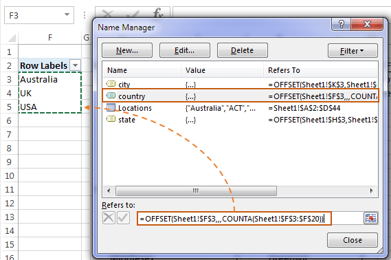
The dynamic named range formula for the Country data validation list is fairly straight forward:

=OFFSET(Sheet1!$F$3, , , COUNTA(Sheet1!$F$3:$F$20))

In English it reads:

Start the range in cell F3, , , then count the values in cells F3:F20 (F20 allows for growth) and use the resulting value as the height of the range.

Note: The 2 empty arguments denoted by , , account for the rows and cols arguments we don’t need.

The COUNTA part of the formula returns 3 and so the result returned by OFFSET is a range 3 rows high, which is F3:F5

In the image below we can see the formula in the Name Manager (Formulas tab or F3 to open the Name Manager), and the cells F3:F5 in the worksheet are surrounded in marching ants to show the range returned by the ‘country’ name:

Helper Cells

For the State and City named ranges we’ll use some helper cells to provide OFFSET with the rows and height arguments for the Country and State.

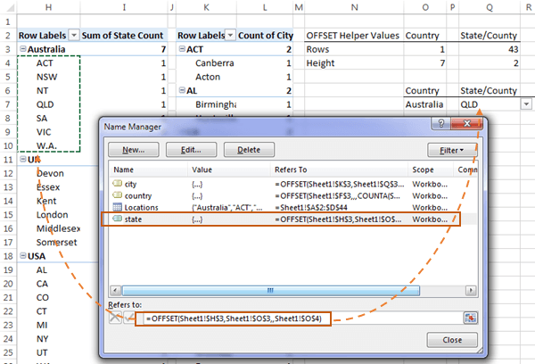
Let’s start with the dynamic named range for ‘state’, which uses this formula:

=OFFSET(Sheet1!$H$3,Sheet1!$O$3,,Sheet1!$O$4)

The reference argument is H3, which is the first row (after the header) of the second PivotTable. The rows and height arguments are referencing helper cells O3 and O4 respectively.

Rows: Cell O3 contains a MATCH formula that locates the row number in the range H3:H40 that contains the country selected in the first data validation list.

Height: Cell O4 contains an INDEX formula that returns the state count for the country selected in the first data validation list.

Below is an image showing the helper cells (O3 and O4) and the formulas contained within:

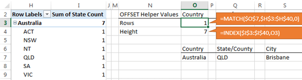
We can see in the image above that the country selected is Australia, which is in the first row of the range H3:H40, so MATCH returns 1.

In cell O4 INDEX references helper cell O3 to return the 1^st value in the range I3:I40, which is the 7 in cell I3.

OFFSET uses 1 as the rows argument and 7 as the height argument and the dynamic named range formula evaluates to:

=OFFSET(Sheet1!$H$3,1,,7)

Which evaluates to the range:

=H4:H10

And when this named range (state) is used as the source for the data validation list we get a list of Australian states because ‘Australia’ is selected in the Country data validation list in cell O7:

The dynamic named range formula for ‘city’, which is used as the source for the City data validation list, works similarly:

=OFFSET(Sheet1!$K$3,Sheet1!$Q$3,,Sheet1!$Q$4)

It references helper cells Q3 and Q4 which locate the state in the third PivotTable and number of cities for that state using the same technique as the State named range.

Notes:

• If you’re confident with OFFSET and dynamic named ranges you can nest the formulas from the helper cells into the dynamic named range formula if you prefer.
• If you have more dependencies you can replicate the dynamic named ranges accordingly.

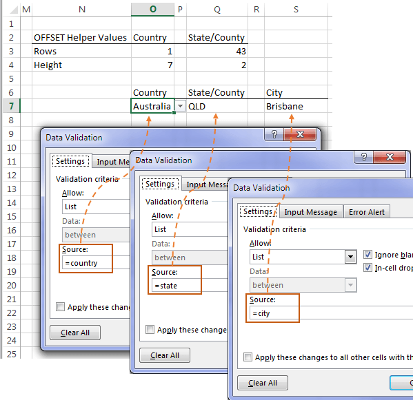
4.      Data Validation Lists

Now all that remains is to set up the data validation lists in the cells you want and use the named range as the ‘source’.

On the Data tab > Data Validation. In the ‘Allow’ field choose ‘List’ and in the ‘Data’ field enter your dynamic named range:

Limitations

1. If you have States or Cities that are present in multiple countries/states then you have to make them unique. For example, both USA and Australia have a WA state. In the US, WA is for Washington and in Australia, WA is for Western Australia. I’ve entered WA for Australia as W.A. to differentiate it. *Update - see solution to this limitation below

2. This only works for one set of Data Validation Lists. If you want to copy the Data Validation lists to multiple rows then you'll find a similar technique in this Excel workbook.

Duplicate State/City Solutions

Update

A few of our members took on the challenge of solving the duplicate state/city limitations and they agreed to let me share them with you here.

1. Andrew Evans used a simple COUNTIFS to ensure the country and state matched in step 1. He also had to make some other changes and you can see them all in his file here.

2. Jim Benton avoided step 1 altogether by shifting the count outside of the PivotTable. You can see his file here.

3. Leonid Koyfman used an array formula and the seldom used N function to perform a logical test inside MATCH. He also added some Conditional Formatting to highlight when the State or City lists didn't match a selection higher up. You can see Leonid's file here.

4. Henk Huiting has a slightly different approach which also allows for use on multiple rows and returns an error if you try to choose a different item before clearing entries downstream. You can see it here.

Thanks

I love to see this amazing Excel community working together to find solutions that we can all learn from. Thanks to Andrew, Jim, Leonid and Henk for taking the time to share your ideas.

A big thank you to PaulaS and UtterAccess for this awesome technique. PaulaS shared a link on our Excel Forum to this technique on the UtterAccess.com wiki.