The OFFSET function is one of Excel’s best kept secrets. Probably because it’s quite tricky to explain, and can be confusing to understand.
In this tutorial I’m going to do my best to keep it simple so you can get your head around it and then I'll cover a few of the most useful ways I find to use OFFSET. I'll also show you the things that trip people up, so you can troubleshoot when OFFSET isn't returning the range you expect.
Table of Contents
OFFSET Function VideoDownload the Example File
Technical Explanation
Things you should know
OFFSET Function Examples
OFFSET Function Practical Uses
Common Mistakes
Watch out for Volatility
Watch the Video

Download the Workbook
Enter your email address below to download the sample workbook.
Excel OFFSET function technical explanation
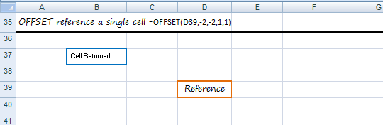
The OFFSET function returns a cell or range of cells that are a specified number of rows and columns from the original cell or range of cells.
The OFFSET Function Syntax is:
=OFFSET(reference, rows, columns, [height], [width])
I like to think of OFFSET a bit like a treasure map. The spot marked ‘X’ can either be a single cell or a range of cells (more on this later).
In our example let’s say our starting point is cell A1 and the spot marked ‘X’ is cell D5.
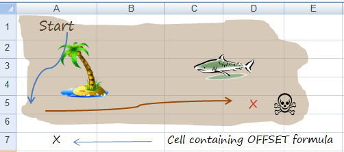
So in treasure map speak our OFFSET function would read:
=OFFSET(starting at A1, step down 4 rows (you’ll be in cell A5), then step across 3 columns (you’ll be in cell D5), Including cell D5 you’ll find the treasure in a range that’s 1 cell high, and one cell wide i.e. cell D5 )
And we would write it in Excel like this:
=OFFSET(A1,4,3,1,1)
Let’s break it down into the arguments:
=OFFSET(reference,rows,columns,height,width)
1) The reference is the starting point in your treasure map/worksheet.
2) Rows are the number of rows you want Excel to move from the starting point.
3) Columns are the number of columns you want Excel to move from the starting point.
4) Height is the number of rows ‘X’ occupies, in our example it's 1.
5) Width is the number of columns ‘X’ occupies, in our example it's 1.
Things you should know
- You can enter the OFFSET formula in any cell, except of course the cell/cells where ‘X’ is. In the above example our formula is in cell A7. Although in this example it returns the value in cell A7, it isn’t actually designed to use on its own, but because in this example we’re asking OFFSET to only return 1 cell, it returns the value in the cell. If we asked it to return a range of cells it would return an error in Excel 2019 and earlier. In later versions of Excel with Dynamic Arrays it would spill the results.
- The reference can be a single cell or a range of cells, likewise the result OFFSET returns.
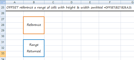
- The height and width arguments are optional, if you don’t enter a height and width it will return a range that is the same height and width as the reference.
OFFSET Function Examples
Practical Uses
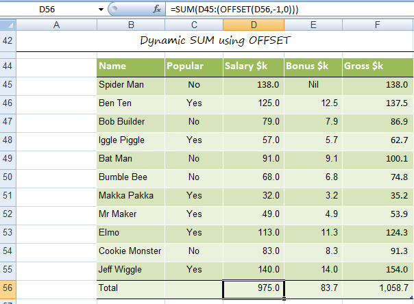
1) Create a Dynamic SUM Formula
How often do you have to update the range of a SUM formula because you’ve added a row just above the SUM and it hasn’t automatically picked it up? It's less of an issue with newer versions of Excel, but it does still happen, so here’s how I use OFFSET to save time by making my SUM formulas dynamic.
In the table below I have Totals in row 56. In cell D56 my SUM formula using OFFSET would look like this:
=SUM(D45:(OFFSET(D56,-1,0)))
2) Use OFFSET and MATCH functions together with SUM and MAX
There are a few things going on in the example below:
I. In Cell B61 there is a drop down list or data validation list as they’re called in Excel.
By changing the selection in cell B61 my formulas in cells B62 and B63 dynamically change to give the SUM of the viewers for the selected program and the MAX viewers.
Since I already covered SUM with OFFSET above, I’m just going to cover the OFFSET and MATCH section of the formula in the example below.
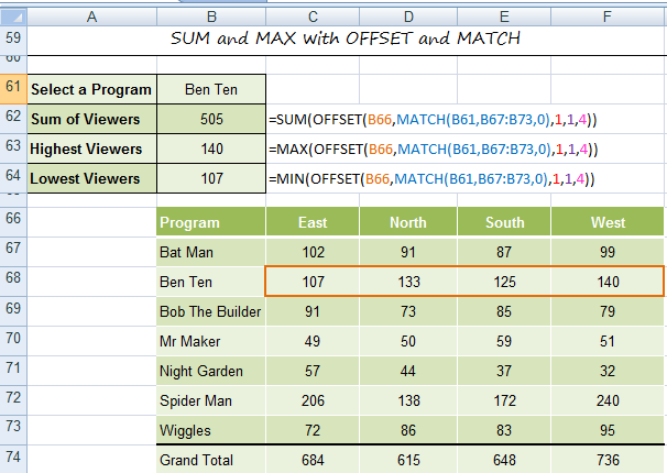
II. Working through the ‘Sum of Viewers’ formula, the reference cell for the OFFSET function is B66, i.e. the junction of the table.
III. We then use the MATCH function to find the row that Ben Ten is on from the range B67:B73, with row 67 being 1, row 68 being 2 etc. This result is then used to instruct the OFFSET function how many rows from B66 Ben Ten is on. In this case it is 2.
IV. We then use 1 as the number of columns so that the start of the SUM is from column C.
V. The number of rows in our range we want summed is 1
VI. The number of columns in our range we want summed is 4.
VII. The MAX and MIN formulas for the Highest and Lowest Viewers works in the same way, only instead of SUM we used MAX and MIN.
3) Dynamic Named Ranges for Charts
Another common way to use OFFSET is to create dynamic named ranges. For example, below I have a table of data that I’ve charted. As I add years to the table, I want the chart to automatically pick up the new data.
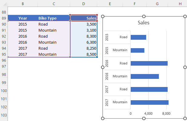
I need two defined names, one for the axis labels and one for the values.
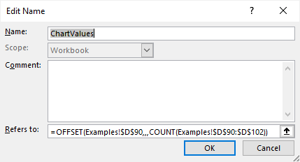
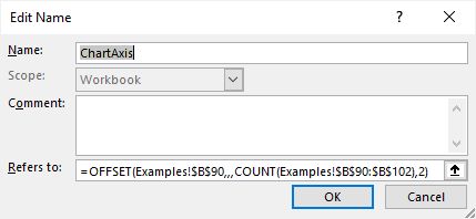
Then edit the chart data source (right-click chart > Select Data > Edit) and insert the names:
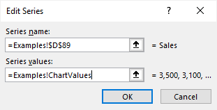
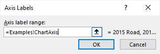
IMPORTANT: the names must be prefixed by the sheet name followed by an exclamation mark.
Common Mistakes
There are two common mistakes people make with OFFSET and I get emails about these issues all the time. They’re super easy to spot when you know the cause.
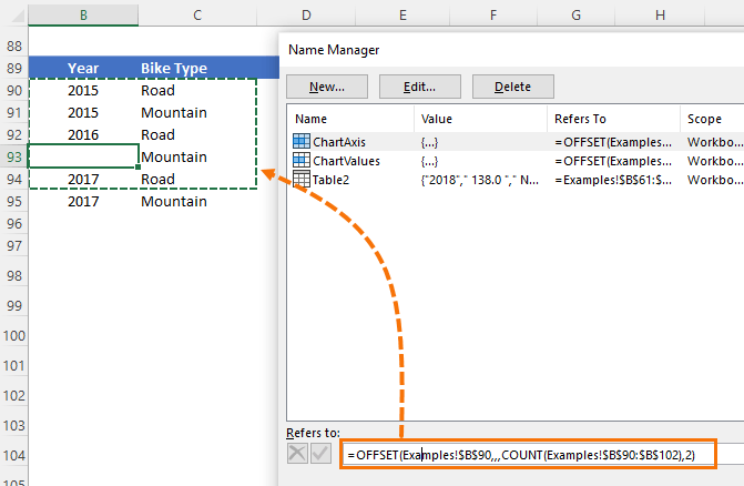
The first mistake is using COUNT or COUNTA to return the size of a range, except there are blanks scattered in the range being counted. We can see in the name manager below that the OFFSET range is one row short, which is caused by the empty Year cell:
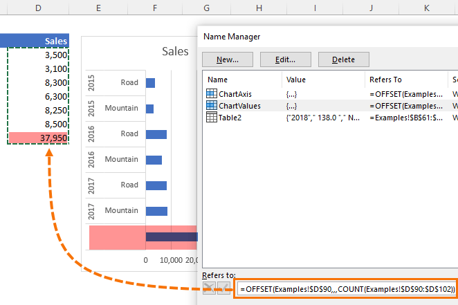
The second mistake is entering data in a range that’s being counted. For example, it's quite common to use a cell under your table to do some quick math not realising that that cell is part of a range being counted by offset:
So, if your offset formula is returning the wrong range the easiest way to check is to open the name manager and check the range being returned. If the range is too short then you've probably got blanks being counted, and if your range is too long then you've probably got some erroneous data lingering below your table that's being included.
Watch out for Volatility
One last word of warning is that OFFSET is a volatile function, which in simple terms means it recalculates more often than most functions which are not volatile. The bottom line is that OFFSET can potentially result in performance issues if you use it too much in a file. However, if you’re using it to generate dynamic named ranges and the like then it’s not likely to cause you any problems. Just don’t go entering it in an entire column of a table.

Thank you for this really good understandable explanation.
Hi Mynda,
I get stuck on this formula:=OFFSET($C$5;;;COUNT($C$5:$C$13);2) —> it resulted “VALUE”(error), I use ms.office 2019. Can you please advice?
Thanks
There is nothing wrong with the formula itself, so it must be something it’s referencing. Please post your question on our Excel forum where you can also upload a sample file and we can help you further.
i can see that offset also takes decimal values, how does that work?
OFFSET ignores the decimal component of the value. i.e. 1.6 is treated as 1.
Hello,
Can you help what this code does please?
For j = 0 To 10
Range(“FilePath”).Offset(4 * j, 0).Value
Next j
Hi Sarah,
Please post your question on our Excel forum where you can also upload a sample file and we can help you further.
Mynda
Hi Mynda, another great article. I’m editing some of my ancient formulae to use OFFSET: don’t know why I didn’t use it earlier!! The data I’m working on is in a Table. I’m adding new rows at the bottom of the Table more often than inserting a new row in the Table. I’m constantly editing the Applies to range list as a result. My query: would OFFSET be useful when defining a Conditional Format range for a given column? I notice XL converts formulae to an absolute range in the CF manager. Would using INDIRECT() be any better? Are there any other options? rgds
Hi Steve,
If you add a new row in the very next row under a table it will automatically include it in the range, so there’s no need to edit anything that references the table. This is more efficient than writing OFFSET formulas. Conditional Formatting will automatically grow with the table as long as you apply the formatting to the whole column when you set it up.
Mynda
Regarding your use of SUM() and OFFSET(), I usually go a step further to ensure a row added to the top of a “table” works, too.
Your example: =SUM(D45:(OFFSET(D56,-1,0)))
My extra-cautious approach: =SUM(OFFSET(D44,1,0):OFFSET(D56,-1,0))
Keep up the good postings!
Good to keep in mind if that scenario is likely in your data. Thanks for sharing, Dave!
Concerning OFFSET and SUM and MAX in exercise 2): A shorter alternative would be, for example:
=SUM(XLOOKUP(B75,B74:B80,C74:F80))
Yes, if you have Excel 2021 or 365 you can use XLOOKUP.
Or FILTER which is even shorter than XLOOKUP:
You can also use INDEX in any version of Excel:
Mynda
Amazing post. Extremely easy to follow.
Thank you, that’s great to hear!
Hi
I too like to check that totals add up correctly. However, the method I use puts the check in a cell that is part of the analysis itself as opposed to using another column.
Using my method with example 3 above, I would enter the following formula in cell A86
“=IF(SUM(F79:F85)=F86,”Grand Total”, “Out of Balance”).
Having read you excellent explanation of the OFFSET function my formula now becomes
“=IF(SUM(F79:(OFFSET(F86,-1,0)))=F86,”Grand Total”,”Out of Balance”)”.
Unfortunately, I guess that by omitting the use of the COUNT function, it now becomes just another way of using SUM with OFFSET; a la example one. Hope you don’t mind another perspective.
Regards
Thanks for sharing, Valence! Always nice to have another perspective 🙂
Hi,
Thansk for awesome explaination.
I am using offset +match with drop down list but i am getting error as below.
So when i select Jan month via drop down , out put i am getting is Jan – which is correct but when i chagne to feb month in my dropdown, output i am getting is “JAN”, “FEB”
Please advise.
MONTH productivity Target
JAN 28 95 Month FEB MONTH JAN
FEB 47 98 productivity FEB
MAR 54 99 Target
APR 68 98
MAY 85 92
JUN 75 91
JUL 85 99
AUG 88 99
SEP 68 98
OCT 78 92
NOV 65 91
DEC 88 95
Thanks
Kavita
Sorry, forgot to mention formula i have applied.
please see below
=OFFSET($A$2,0,0,MATCH(F$2,A$2:A$13,0),1)
=offset (where my offset formula starts in the range, 0,0, match (dropdown list, first column of the ragne, 0), 1)
pls advise
Thanks
Kavita
Hi Kavita,
What should the function return, you did not mentioned which is the expected output?
If you want to get the same month as the dropdown selection, you should use:
=OFFSET($A$2,MATCH(F$2,A$2:A$13,0),0,1,1)
Hi Catalin,
i tried with formula above and i am getting output as “FEB” if i select “JAN” from dropdown instead of “JAN”
For “FEB” from dropdown, i am getting out put as “MAR”
not sure why.
pls assist.
Hi Kavita,
Try this:
Mynda
Perfect, thanks heaps
I just have to say THANK YOU so much for this post!!! I modified the math a bit to suit my needs but this is just awesome. Great explanation!
So pleased it was helpful, Adrienne!
Is the 5 parameter offset command still an acceptable command in VBA? All I can get out of it is errors- which is about all I ever get from VBA! I feel like i need to give up. OR is it a part of 365 – I quit using 365 and OneDrive due to it loosing all my files and sticking them where it wanted to. I could NOT find anything about it on Microsoft Docs.
Hi Carl,
VBA has is own OFFSET property which you use on ranges e.g.
Range(“A1”).Offset(2,5).Select
Will select F3.
https://docs.microsoft.com/en-us/office/vba/api/excel.range.offset
Regards
Phil
Thank you. Offset explanation was good.
Thx 🙂
class students are as A B C D E F G H I J K up to z . they came everyday but someday individual students absent,
student B and student H are close friends . B and H also not attend every day someday B attended someday H attended. in Excel sheet attended days are marking in individual cells in columns a row for each student. let me know a formula how to count days of both student together B and H attended not individually. if B or H absent one day that leave that day without count.
Hi Ibrahim,
Please upload a sample file with your data structure on our forum, it will be easier for us to understand your problem and to provide a solution built for your data structure.
Great…Clear explanation.
Thank you…
I often use OFFSET to define a named range so I don’t have to consider if rows or columns have been added. For instance,
OFFSET(A2,0,0,COUNTA($A:$A)-1,5)
where column A has data, but an unknown or variable number of rows with the first row being headings, and there are five columns of data in the range.
finally I understand offset
Yay! Glad I could help 🙂
Great explanation – thank you
Thanks! Glad you found it useful 🙂
Good
A super useful article even for a such complex function to understand… Thanks!!!
Thank you! Glad we could help.
Excellent
Thanks!
Phil
I am using Excel 2013 and when I add a row just above the cell containing SUM formula, it automatically picks the cell added. So I think OFFSET is not necessary in this case, right?
Hi Lam,
I wouldn’t rely on formulas always updating as they should unless you put your data in an Excel Table.
Mynda
Outstanding tutorial!!!! Simple to understand and thanks loads for the practice worksheet – totally brilliant!
🙂 Thanks, Lesley. Glad you found it useful.
Mynda
If I have a table with each month as a column and when I update a month(column), can I still update range select by using OFFSET?
eg. Mon Jan Feb Mar Apr .+New Month..
Value 5 10 8 9 .+Value..
Hi Rui,
Yes. Have you tried it?
Let me know if you get stuck.
Mynda
The value of say F5 is 120.
A1=the value of F5.
is there a formula that i can use that will place the value of F5 all the way to “row” 120? In other words what ever the value of F5 is, as it will change, i want that number of rows in Column 1 filled with that value. Is that possible?
Hi Wendy,
You could use IF to do this. e.g. in cell A1:
You'll have to copy the formula down more than enough rows to allow for the maximum value in cell F5. Any rows > the value in F5 will contain a blank.
Mynda
Your explanations are fantastic and give great insight to what ALL these functions are useful for and in terms that can be understood – Thank you so much for taking the time to make these valuable tutorials!
Thank you, David. I’m happy you find our site useful 🙂
Mynda
Hello!
Could you help me create an offset for this formula:
=SUM(‘Awards Original’!B456) =SUM(‘Awards Original’!B458) =SUM(‘Awards Original’!B459) =SUM(‘Awards Original’!B460) =SUM(‘Awards Original’!B461) =SUM(‘Awards Original’!B462) =SUM(‘Awards Original’!B463) =SUM(‘Awards Original’!B457)
=SUM(‘Awards Original’!B467) =SUM(‘Awards Original’!B469) =SUM(‘Awards Original’!B70) =SUM(‘Awards Original’!B471) =SUM(‘Awards Original’!B472) =SUM(‘Awards Original’!B473) =SUM(‘Awards Original’!B464) =SUM(‘Awards Original’!B468)
=SUM(‘Awards Original’!B478) =SUM(‘Awards Original’!B480) =SUM(‘Awards Original’!B481) =SUM(‘Awards Original’!B482) =SUM(‘Awards Original’!B483) =SUM(‘Awards Original’!B484) =SUM(‘Awards Original’!B485) =SUM(‘Awards Original’!B479)
Each one is basically 11 rows down from the last.
Seeing the original and the new with offset helps, but I’m still missing out on something in my wee little head.
Thank you!
Hi Kim,
Can you please prepare and upload a sample file with more details on what you are trying to do? You can use our Help Desk to create a new ticket: Help Desk
It will be a lot easier to understand your situation, thanks for understanding.
Catalin
When I try to download a workbook (in the case for Offset) my screen shows a bunch of code, and I do not know how to download it, or if I did, what to do with it to make it look like a workbook. Please suggest a remedy.
Hi Arthur,
Sorry you’re having trouble downloading the workbook. Please right-click the download link > File Save As (or equivalent on your browser) > make sure the file extension is .xlsx in the File Name field > save. Then you can nagivagte to the folder where you saved the file and open lik you would any other Excel file.
Let me know if you still have problems.
Kind regards,
Mynda
You don’t need the “,0” to make the formula work. In fact the “,0” could be any number and it does not change the outcome.
I would say that the zero is “sue-perfer-loo-us.”
=SUM(OFFSET($B$66,MATCH($B$61,$B$67:$B$74,0),1,1,4))
=SUM(OFFSET($B$66,MATCH($B$61,$B$67:$B$74),1,1,4))
Ted
Hi Ted,
If you refer to the last Argument of the MATCH function, you are right, it is optional, and the default value is 0 (Exact Match). Only if someone does not need an exact match should choose from 1 (or a positive number) (Less Than) or -1 (or a negative number) (Greater Than).
Thanks for your contribution
Cheers,
Catalin
Hey Mynda,
First, thank you for your post. I use OFFSET Function to create various scenarios in my financial models. It works awesome. However, what I haven’t figured out – and I hope, you can help me with – is how to extract the results of those scenarios into a Summary without copy&paste those after having selected the Scenario from a drop-down list.
Thank you in advance.
Best,
Silke
Hi Silke,
Are you able to send me your file via the Help Desk as I’m having trouble visualising what you meany by “how to extract the results of those scenarios into a summary without copy and paste”.
One thing that comes to mind is using a PivotTable to analyse your data and then extracting the filtered items to separate sheets, as described here: https://www.myonlinetraininghub.com/excel-pivot-tables-to-extract-data
Thanks,
Mynda
It is really helpful.. even for a person who is not from sales or finance background. these blogs are really helping me to enhance my skills to next level.. Really thanks Mynda 🙂
Thanks, Warisha. I’m glad we can help 🙂
Hi,
Is it possible to use an offset within a sumifs. My sumifs formula works but I want to offset it by 4 rows…is this possible
Replace the range, like: A1:A100 for example, with: OFFSET(A1:A100,4,0)
Catalin
This is formula I learned online. And I do not have to search any further because its been made so easy here. Thanks.
Glad to hear that Jitin, it’s rewarding for us to know that our work is appreciated 🙂
thank you so much for your helpful information.
You’re welcome, Easton.
Hai Madam,
Can you send the detail notes with more examples for Offset, Match and Index Functions
Hi Gudipally,
This tutorial contains the detailed notes I have for OFFSET. You can find a tutorial on INDEX & MATCH here:
https://www.myonlinetraininghub.com/excel-index-and-match-functions
Kind regards,
Mynda
OFFSET($A$13,MATCH($E$12,$A$14:$A$68,0),1,7,1) captures 7 row data. Values can be seen in the Formula Bar by selecting the formula and pressing F9.: {5;6;7;8;9;10;2}.
Question is: How can we have these 7 values in 7 different cells ?
Thanks.
Hi Jitin,
Select 7 consecutive cells, go to formula bar and paste the formula there, then press Ctrl+Shift+Enter. This will enter the formula in all 7 cells, and all 7 results will be displayed on those cells.
Catalin
Thanks a lot!
You’re wellcome 🙂
I created 2 tables:
Table 1 is the source table (main table)
Table 2 is a table which column A and B should be identical to column A and B of table 1.
Table 1 has column A,B,C,D and E
Table 2 has columns A,B (same as table 1 so i used OFFSET formula) columns C,D and E which
are different from columns from table 1
the problem, while I add a new row in table 1 , it will be added to Table 2 but the text
in column C, D and E will not move with its original row as it was related
before adding the new row. the text in column C,D and E will be on the same row
of the new row in case i inserted the new row above.
So how can i able to insert a row on Table 1 and the related text of this row in table 2 will continue to appears on the same row?
Hi Liran,
Please upload a sample workbook with your data structure and details on what you want to do, itwill be easier for us to understand your situation.
You can use our Help Desk system to upload the file.
Thanks
Catalin
Is there a way to use SumIf in the above example (no. 2) instead of using sum,match,offset, or it’s only way doing this.
Regards,
Manish
Hi Manish,
A SUMIF can only sum one column, so no you can’t achieve the same results with SUMIF. That’s not to say the OFFSET example is the only way but it serves as a useful demonstration.
Mynda
Hi Mynda,
SUBJECT : SUM and MAX with OFFSET and MATCH
Where you have used the formula ,=SUM(OFFSET(B66,MATCH(B61,B67:B73,0),1,1,4)))
for calculating the sum of BEN TEN’S viewers, what if we add/have one more row of BEN TEN in the data table, how can we then change the formula to sum up that row too?
Thanks,
Raj
Hi Raj,
Ben Ten Viewers are in columns C,D,E and F (not in rows!) To add one more column with Viewers, just increase the last argument ([width]) of the OFFSET formula, from 4 to 5.
Adding rows to the table means adding a new Program, not viewers to BEN TEN. In case you want to add a new Program (a new row), the only change that must be made is in MATCH formula, to extend the search range with 1 row: from MATCH(B61,B67:B73,0) to MATCH(B61,B67:B74,0)
Hope it helps,
Catalin
Awesome site guys!! 🙂
Question, how can I use the above example to create a “Top 10” or “Bottom 10” list?
In my case, I’m refering my list from a pivot table (which works great), but I’m limited to using Auto Filter to sort from smallest to highest. Which isn’t all that great as every time the subject changes to provide a new list, the filtering resets.
Might help if I added the formula I used:
This formula returns the list:
=OFFSET(True_Pivot!H14,MATCH($M$2,True_Pivot!$I$11:$I$234,0),$T$3)
This one returns the “grade”:
=OFFSET(True_Pivot!I14,MATCH($M$2,True_Pivot!$I$11:$I$234,0),$T$3)
Hi Rhett,
Thanks for your kind words 🙂
If you’re already using a PivotTable why don’t you just use the filters in the PivotTable to create your top 10/bottom 10 list?
Right click the field you want filtered > Value Fitlers > Top 10
Let me know if that doesn’t work for you.
Kind regards,
Mynda.
Hi,
I would like to “transfer” (= show somewhere else) content of my columns based on P_name header (e.g. if P1, transfer A,B,C; if P4, transfer L,M,N).
P_name P1 P2 P3 P4
content A D G L
B E H M
C F K N
I tried to use OFFSET/MATCH formula, but it is showing this formula contains an error: =OFFSET(MATCH(header,P_name,0),1,0)
Any idea, what I am doing wrong?
I can see the problem, if I enter it as an array formula that I get always values from first row only, because my OFFSET formula defines row 1 from the reference. How can I force the formula to “adjust” rows in an array format?
Thanks,
Peter
Hi Peter,
The MATCH function returns a value, e.g. 1 or 2 or 50. The OFFSET function requires a cell reference as it’s first argument. This is why you’re getting an error.
A better formula would the INDEX & MATCH as OFFSET is volatile where as INDEX isn’t.
Kind regards,
Mynda.
Thank you, Mynda, these are the nuances I don’t realize by reading some instructios. Peter
You’re welcome, Peter 🙂
Very “Simply” explained..
Thanks, Aniya 🙂
Hi Mynda,
I would like to team up OFFSET formula with ABS formula. Is this possible?
thx
Thomas
Hi Thomas,
Yes, possibly. It depends in what context. Do you have an example file you can send me via the help desk that shows what you want to do?
Mynda.
Unfortunately its a big file with much irrelevant but confidential stuff in it.
The problem formula is quite simple though; its a simple row of numbers from which i need an average. I use OFFSET to keep it flexible with the number of months passed.
=SUM(ABS(OFFSET(J26;0;W26;1;$X20)))/$X20
This returns an error, thankfull for any ideas..
br
Thomas
Hi Thomas,
Is the OFFSET just returning one cell or multiple cells? If multiple then try putting the ABS outside the SUM, like this:
If that doesn’t work it would help to know the values in W26 and X20.
Kind regards,
Mynda.
Hi Mynda,
Thank you for your suggestion.
Unfortunately this only provides an absolute value of the total after adding both plusses and minusses.
The offset formula was taking 1 row and 5 columns, i.e. 5 cells with both positive and negative numbers, and i wanted an average of the total regardless of foresign. (values W26 = 2, X20 = 5)
I played a bit around and the following formula seems to work.
=SUMPRODUCT(ABS(OFFSET(J26;0;W26;1;$X20)))/$X20
To be honest i am not sure why the sumproduct functions works for me though 😉
br
Thomas
Hi Thomas,
Ah, now I understand that the OFFSET returns more than one cell it makes more sense.
The reason SUMPRODUCT works is because it can handle arrays. So, the OFFSET function returns an array of 5 cells, which are then fed to the ABS function which strips out the negative signs, and SUMPRODUCT then adds them up.
You can read more on array formulas here (SUMPRODUCT is an array formula however you don’t need to enter it with CTRL+SHIFT+ENTER like typical array formulas.
And more on SUMPRODUCT here.
I hope that helps.
Kind regards,
Mynda.
Hi Mynda
I need to find the max value in a column and then get the date corresponding from the same row a few columns back.
Tried ‘-> =offset(max(I3:I936),-8,0)
Gives an error – could you advise?
Peter
Hi Peter,
You can use INDEX and MATCH for this:
Kind regards,
Mynda.
Hi. When using the offset formula, can I then “offset” from a Hlookup point? Something like this =OFFSET(HLOOKUP….)? Its because my reference point can be different, depending on a dropdown menu.
I have this sheet where I have a lot of data – lets call it the “archive sheet”. Then I have to extract some data depending on which year I choose.
Hi Lars,
No, you can’t use the HLOOKUP to return the cell reference for OFFSET because HLOOKUP returns the value in the cell you’re looking up, not the cell address or reference which is what OFFSET needs. But you can use the INDEX function to return the cell reference.
INDEX and MATCH together can work in the same way as VLOOKUP or HLOOKUP. More on INDEX & MATCH here. e.g.
Note: you can also use MATCH to return the row number you want returned. So it would be an INDEX, MATCH, MATCH formula 🙂
I hope that helps.
Kind regards,
Mynda.
Mynda, hello
Your training site is very helpful in explaining the offset concept and its application. For the problem I am trying to solve I tried using your response to few of the questions which come close to mine, however it did not work.
Let me explain the Excel problem I have:
I have two worksheets in my work book. Worksheet A and Worksheet B.
Worksheet A has 10 sections with 10 rows each. Column A for each of the 10 rows in the sections has “add question here” as the content. There are other columns in the sections that have formulas in them. I have a macro that is executed by a button in this sheet which basically adds a row above the last row in each of the 10 sections based on placement of cursor.
Worksheet B is a summary of the 10 sections in Worksheet B. There is a formula in this worksheet that counts the rows in each section using the Count A function. My issues is that when my macro in worksheet A adds a new row, the formula for Count A does not update the row count
Your assistance will be greatly appreciated.
Regards
Hi AAB,
Perhaps you can send me your workbook via the help desk, as it would be easier to put a custom solution in it than try to explain it in the comments.
Kind regards,
Mynda.
Thanks for the info. Always nice to add useful tools to the toolbox.
Since this is my first introduction to this function, I have not used it yet. But I think I can apply this to a rolling 4 quarter (or rolling 12 month) drug cost (or utilization) summary and then graph those results. I really like the combination with =match() and a drop down list. I can then provide a dynamic tool for clinical pharmacists to graphically review utilization and cost over time for any therapeutic class of medications. They can scroll through each class using the drop down.
Clearly, the key to effectively applying =offset() is in how you have the data arranged. You really need to know your end result before you arrange the initial table.
Very powerful function…
Very cool!
Thanks!
Hi Andy,
Sounds like you’ve got some great ideas for using the OFFSET function.
Thanks for sharing.
Mynda.
Thanks a lot more grees to your elbow
Thanks, Jazuli 🙂
Thanks Mynda. Great explanation of OFFSET, it’s all clear now!!
🙂 Thanks, Simon. Glad I could help.
Hi,
Thanks very much for your very informative and very detailed explanations on excel functions. On your table above,on using OFFSET,MATCH, SUM,MAX/MIN, functions, how do you set the same formuals (sum,max & min) to select Bat man instead of Ben ten, ie select the program as Bat man and insert the formulas that will give sum of viewers, highest and lowest viewers, as you have done for Ben ten.i have tried this but its not working out.
Regards
Simba
Hi Simbarashe,
The formula is referencing cell B61 which contains ‘Ben Ten’. To change the formula to return results for Bat Man you can either type ‘Bat Man’ in cell B61 or replace the reference to B61 in the formula with “Bat Man” (including the double quotes around Bat Man).
Like this:
=SUM(OFFSET(B66,MATCH("Bat Man",B67:B73,0),1,1,4))Kind regards,
Mynda.
hi,
I have done a table like the one below using your data;
Program Bat man Ben ten Bob the marker …………..
Sum of viewers
Highest viewers
Lowest Viewers
So i wanted to complete it using sum, max and min with OFFSET & MATCH but it is skipping Bat man. Instead the formula is putting the data for Ben ten on Bat man, Bob the marker on Ben ten, and so on.
Please help.
Regards
Simba
Hi Simbarashe,
I recommend you use the Evaluate Formula tool (Formulas tab of the ribbon > Evaluate Formula) to inspect the formulas and troubleshoot where you’re going wrong. If you’re still stuck you can send me the file via the help desk.
Kind regards,
Mynda.
Excellent explanation of offset function
Thank you, Zikica 🙂
I have an amortization spread template with an x & y axis graph that can go anywhere from say, 5 to 10 yrs for a loan amortization. While I can readily adjust the graph for different amortizations, I have a department that works for me that are not near as conversent on Excel. So I need a way to make the graph “range” dynamic and adjust to the changing amortization periods. I have read the above OFFSET explanation and think that it may be useful, but I can’t seems to intergrate it into a “range”. Any suggestions
Hi Ralph,
When you use a dynamic named range as a source for a chart you need to also include the worksheet name in the axis label range. For example:
=’Sheet1.xlsx’!dynamic_named_range
If that doesn’t solve your problem perhaps you’d like to send me your file and I can take a look.
Kind regards,
Mynda.
best document of excel offset function
Thank you, Gulimtiaz 🙂
Hello,
You claim that the OFFSET() function can return a range of cells. Can you show me how that can be done. So far it only returns the value in one cell. I would like to know what function can return a range of cells in the form A4:B16 for example.
Hi Tosin,
If you enter OFFSET in one cell but the formula is returning a range of cells Excel can only display the first value in the range since you only entered the formula in one cell.
If you wan’t OFFSET to return the values from a range of cells (as opposed to passing that range to another formula) then you first have to select the number cells you need. i.e. if you want to return a range that is 5 cells high then you first need to select 5 cells, say D1:D5, then you enter your OFFSET formula in the active cell (D1) say, =OFFSET(A1,,,5) and press CTRL+SHIFT+ENTER to return a multi-cell array. This will enter the 5 values in cells A1:A5 in cells D1:D5.
I hope that helps.
Kind regards,
Mynda.
I have used offset mutiple times but adding with match..! wonderful
Thanks, Kamran 🙂
Hi Mynda
The Examples given are really nice.
But can you Please share how can we use offsets in Charts. I want to present the data of 15 days in line graph and want when ever I insert a new column for a new date my oldest date should be removed from the chart. I insert a new column in the beginning of the workbook. I want the range to be fixed.
example- I have fixed the range of my chart from column ‘D’ to ‘I’ and if i insert a new column ‘E’ then ‘J’ column which was earlier ‘I’ should not be shown in graph.
Please Help. Thanks
Hi Khushboo,
Please send your file please here : HELP DESK.
Cheers,
CarloE
I love you.
I raked my brains trying to get an average with a variable range that depends on the month we are in, for a spreadsheet that tracks expenses. I read several other forums, tutorials, and explanations, but I couldn’t figure it out until I read your page.
How did I use it? I have one column (F) where I want the average to show, and twelve columns for expenses, one for each month, with entries that start at row 7. But what I want is the monthly average to date, and AVERAGE() spreads it over 12 months, so there came OFFSET() to the rescue, and this is what I did:
=AVERAGE(OFFSET(F7,0,1,1,MONTH(TODAY())))
But I didn’t want the partial expenses of the current month to skew my averages, so I added a -1 after the month:
=AVERAGE(OFFSET(F7,0,1,1,MONTH(TODAY())-1))
The problem I have now is that it will never include December. So I introduce an IF():
=IF(MONTH(TODAY())=1,AVERAGE(G7:R7),AVERAGE(OFFSET(F7,0,1,1,MONTH(TODAY())-1)))
If the condition MONTH(TODAY()), average will be of the whole year, which is what we want to see when we open a spreadsheet of last year book-keeping.
Thank you so much!
Hi Xavier,
You’re welcome on behalf of Mynda!
Keep on sharing.
Cheers,
CarloE
Hi, well done, but I have a question please.
The formula =SUM(OFFSET(D$1,(ROW(B1)-1)*5,0,5,1))
assumes that:
this formula is in Cell B1 (pasted down), and your data is in Column D starting at 1.
What if the data is from G2 downwards, what values should be changed please? And I want the results from B2 downwards.
Thanks!
Hi Beckett,
The only thing you need to change here is the reference which is D$1 to G$2.
So the formula now is:
Cheers,
CarloE
Send a complete copy of excel functions
Hi Enessy,
Here’s the link:
Excel Functions Tips and Tricks
Cheers,
CarloE
Your article help me a lot!, Thank you!.
Hi KSN,
You’re welcome, On behalf of Mynda.
Cheers,
CarloE
Great explanations and examples! The color coding really helps! Please tell me that you’ll be writing all the MS help articles from now on! Lol
Hi Beth,
You bet Mynda will.
Thanks for your words.
Cheers.
Carlo
I find the explanation is very effective and helpful. I am the first time user of this site and presently working on Pricing file, I faced difficulties while using the rank function, in trying to rank the sales and margins of various products within the Product family – eg. we have over 200 product families and within each family on an average 50 Item numbers, all in one worksheet – I need to rank the sales and margin of individual items within the family – can you suggest how to achieve this without specifying the Rank formula for each family.
Thanks
Hi Saurav,
Will you kindly please elaborate this further. Please send your file through Help Desk.
I just want to know what exactly you want.
Perhaps you can try LARGE or SMALL functions.
Cheers.
CarloE
Well written explanation of OFFSET’s use.
I use OFFSET primarily for dynamically creating a data validation list.
I encountered an error, however and have not seen anyone speak to it. I created the following data validation list in an xlsx workbook using Excel 2010. The drop-down works as expected. When I open the same workbook in Excel 2007, there is no drop-down and the data validation list is set to “any value”.
An error appeared in 2007 stating an OFFSET could not be used to address areas on other worksheets. Unfortunately, there is no way around it. Any ideas?
=OFFSET(Clients!$A$1,MATCH(Summary!$A$1,Clients!$A:$A,0)-1,1,COUNTIF(Clients!$A:$A,Summary!$A$1),1)
Hi Dave,
Please send your file to HELP DESK.
At any rate, I tried to simulate the dynamic range using your offset function, And the only time
I got the error was when there were no data yet. Exactly, as you described it; that is, the data validation
list is set to “any value”. After I have reset it, the error doesn’t occur anymore.
Cheers.
CarloE
Yours is the 5th example I read, including excel forums. All I needed was the first example of the treasure map to understand. Once I did, I kind of felt stupid for how simple it was. And that is the genius of a great teacher!
Thank you. Thank you. Thank you. !
Wow, thanks, Serena 🙂 Glad I could help.
AWESOME FORMULA! I was trying to figure out a way to capture data dynamically in a pivot table. I was currently using a named range, but then it made the file large because of the empty cells it was capturing. This eliminates the need to have named ranges. Awesome:-)
Thanks, Shari. Glad we could help you out 🙂
=SUMPRODUCT(OFFSET(A:A,0,MATCH(“Rate”,6:6,0)-1),OFFSET(A:A,0,MATCH(“Qty”,6:6,0)-1))
Can you please explain to me what the purpose is of having -1 at the end of the formula?
Many thanks
Hi LC,
Honestly, I didn’t see the workbook that has this formula.
However, isolating the offset functions which concern your question,
I can see that the column headers at row 6 must have started in column B.
So the maker of this formula had to improvise by deducting 1.
Here’s how this particular offset function works.
        NOTE: Consider the syntax : OFFSET(REFERENCE,Rows to add, Cols to add) hence,
                                    Reference:Row 7, Row 7 + 0, Col A + 5. will give you "QTY"
                                    deducting 1 will give you "RATE" basing on the data below.
The reference is column A.
The row argument is 0, hence, the formula is in any row in column A… let’s just say at row 7.
So the formula is at row 7 where the first data is for the “Rate” and “Qty” columns are.
Hence: Offset(A:A,0… (zero).
The column argument uses the Match Function. It is looking for “Rate” in the
column headers at row 6. Now… to answer your question. Why -1?
Consider the data below. The first column header is at column B, and
the formula uses 6:6 reference to represent all of the column at row 6.
In other words, It started counting from column A… so if you isolate
MATCH(“Rate”,6:6,0) this will return 5. Now if you put 5 in the Offset function:
Offset(A:A,0,5) it means row 7 and col A + 5 or column 6 which will
return “Qty” actually for the Offset Function’s purpose. Hence, the minus 1.
The same goes for the second offset function finding “Qty”.
Try to experiment and isolate the OFFSET and MATCH Function by placing them
in column A.
Read More: SUMPRODUCT
OFFSET
MATCH
Cheers.
CarloE
THANK YOU!
This is a great explanation. I was killing myself trying to figure out what I was doing wrong. It was so simple, ” If we asked it to return a range of cells it would return an error.” No where else I checked made that statement not even Microsoft (unless I missed it in my frustration).
Great work!
🙂 glad we could help, Shelbi.
I tried to use this dynamic offset for COUNTIF and it didn’t work for me. The only time my if would count is if I inserted a row before the last row, not after. But I noted that the count advanced whether I used the dynamic formula or not. Does this only work for SUM?
Hi John,
This will work with countif or any function that accepts a range for an argument.
I replaced the SUM with COUNTIF in the “Dynamic SUM using OFFSET” table under NIL column:
and inserted some with good results.
Please make sure that the range argument of your OFFSET function
should be where your formula is before you insert a row.
In the example, the formulas are in row 56. So make sure,
you must be in the same row. So that when you offset by -1 row; that is,
(i.e. 56-1) 55, your addends should be within the range from 45 to 55.
When you insert a row, your formula will automatically adjusts to 57. Hence,
-1 row, your addends are now within 45 to 56.
I couldn't explain it any better.
Cheers.
CarloE
I’m using the OFFSET function in an Excel gradebook to create easily printed grade sheets for each of my students. I’m wondering if there is any way to bring the cell formatting along with the offset. For example, I hightlight the scores of tasks that were submitted late in the “homework” sheet and am wanting those scores to also be highlighted when they are brought over to the “report” sheet using OFFSET. Thank you!
Hi Debbie,
This is quite challenging; hence,
I used vba so We wouldn’t come out
empty.
Here’s the deal:
1 ALT+F11 (Brings you to the VBE Window)
2 While in the VBE Window, Click Insert, Select Module (Note: not class module)
3 Paste this code:
Sub OffsetColor(rw As Long, cl As Long, YourSheet As String)
    Dim rng As Range
    Dim rLast As Range, iLinkNum As Integer, iArrowNum As Integer
    Dim stMsg As String
    Dim bNewArrow As Boolean
    Application.ScreenUpdating = False
    ActiveCell.ShowPrecedents
    Set rLast = ActiveCell
    iArrowNum = 1
    iLinkNum = 1
    bNewArrow = True

    Do
        Do
            Application.Goto rLast
            On Error Resume Next
            ActiveCell.NavigateArrow TowardPrecedent:=True, ArrowNumber:=iArrowNum, LinkNumber:=iLinkNum
            If Err.Number > 0 Then Exit Do
            On Error GoTo 0
            If rLast.Address(external:=True) = ActiveCell.Address(external:=True) Then
               ' Set rng = Worksheets(YourSheet).Range(Selection.Address)
                '    rLast.Parent.ClearArrows
               '     Application.Goto rLast
               '     MsgBox "Precedents are" & stMsg & test
                '    rLast.Interior.ColorIndex = rng.Cells(1, 1).Offset(rw, cl).Interior.ColorIndex
                Exit Do
            Else
            End If
            bNewArrow = False
            If rLast.Worksheet.Parent.Name = ActiveCell.Worksheet.Parent.Name Then
                If rLast.Worksheet.Name = ActiveCell.Parent.Name Then
                    ' local
                    stMsg = stMsg & vbNewLine & Selection.Address
                    Set rng = Worksheets(ActiveCell.Worksheet.Name).Range(Selection.Address)
                    If rng.Cells(1, 1).Offset(rw, cl).Interior.ColorIndex = xlNone Then
                       Set rng = Worksheets(YourSheet).Range(Selection.Address)
                    Else
                    End If
                Else
                    stMsg = stMsg & vbNewLine & "'" & Selection.Parent.Name & "'!" & Selection.Address
                    Set rng = Worksheets(ActiveCell.Worksheet.Name).Range(Selection.Address)
                End If
            Else
                ' external
                stMsg = stMsg & vbNewLine & Selection.Address(external:=True)
                Set rng = Worksheets(Selection.Address).Range(Selection.Address)
            End If
            iLinkNum = iLinkNum + 1  ' try another link
        Loop
        If bNewArrow Then Exit Do
        iLinkNum = 1
        bNewArrow = True
        iArrowNum = iArrowNum + 1  'try another arrow
    Loop
    rLast.Parent.ClearArrows
    Application.Goto rLast
    rLast.Interior.ColorIndex = rng.Cells(1, 1).Offset(rw, cl).Interior.ColorIndex
End Sub
4 Add a CommandButton. Find it here : Adding a CommandButton from the Developer’s Ribbon
5 Double Click the Button then Copy and Paste the code in the sheet where your offset formulas are.(You may also refer to the link in number 4 on
where to place the codes.) Note: In copying below do not include the Event Procedure Name: Private Sub CommandButton1_Click() and End Sub. It is already provided after you double click.
Private Sub CommandButton1_Click()
    Dim sf As String
    Dim s As Long
    Dim l As Long
    Dim r As String
    Dim c As String
    Dim str As String
    Dim Acell As Range
    Dim Ur As Range
    Set Ur = ActiveSheet.UsedRange
    For Each Acell In Ur
        If CStr(Acell.Formula) Like "*OFFSET*" Then
            sf = Acell.Formula
            s = Application.WorksheetFunction.Search(",", sf)
            l = Application.WorksheetFunction.Search(",", sf, s + 1)
            r = CStr(Mid(sf, s + 1, l - s - 1))
            c = CStr(Mid(sf, l + 1, Len(sf) - l - 1))
            Acell.Select
            Call OffsetColor(CLng(r), CLng(c), "GradeBook")
        Else
        End If
    Next
End Sub
NOTE: “GradeBook” sheet is the assumed name. Replace it with the name of the sheet where your Grades are
6 Put it in Runtime Mode by clicking the “Design Mode” in the Developer’s Tab. You will know that you are in the runtime mode because
your CommandButton is able to be clicked than dragged.
Cheers.
CarloE
Wow – thank you so much! I’ll give this a try today!
Hi Debbie.
On behalf of Mynda and Philip,
I say you’re very much welcome!
Cheers.
Carlo
Hi Mynda:
Excellent coverage of a very confusing topic. I have one question. In the formula COUNT($B$79:OFFSET($B$86,-1,0,1,1)) what does the -1 mean
in the OFFSET portion. I assume it means the cell with last data before the total. You have used the -1 in several examples explaining the OFFSET function .
Hi John,
The -1 instructs Excel to go up or left instead of down or right. Like this:
-1 row would go up one row
-1 column would go left one column
1 row goes down one row
1 column goes right one column
Kind regards,
Mynda.
What is the actual formulae for rearranging the rectangular data values in excel?
I need exact formula for the above function for
A B C
1 One Two Three
2 Four Five Six
Required Ans:
A
1 One
2 Four
3 Two
4 Five
5 Three
6 Six.
Please let me know the operation to do it.
Thanking you.
Hi Karnan,
That’s a good question. Here is a formula you can use (enter in first cell you want your list to start and drag down to copy):
You can thank Roberto Mensa for giving me this solution.
Kind regards,
Mynda.
I want to ask….
How is the function if I want fill :
– A1 with data in C4
– A2 with data in C6
– A3 with data in C8
– A4 with data in C10
– …
Thank you.
Hi Irwan,
You can use this formula:
Copy formula down remaining cells.
Kind regards,
Mynda.
Brilliant!
I just stumbled upon this function without a clue on what it does and what for.
The pirate’s map is by far the best “excel explained” example I’ve seen 🙂
Wow, thanks 🙂
Hi Mynda:
When I try to download the sample workbook, I get a lot of symbols,but
am not able to download anything. Is it possible for you to see if you get the same thing. Otherwise excellent!!
Hi John,
Right click on the sample workbook and then from the menu that appears, choose “Save As”, “Save target” or whatever similar wording is in your menu.
Then make sure the file being saved has the file extension .xlsx
What I think might be happening is that your browser is saving the file as a .zip, Internet Explorer does this a lot.
Regards
Phil
Hi Mynda,
I am really feel very obliged to you for sharing such wonderful information in excel. All tips are so well explained in simple language & I find it extermely useful for anyone however well he/she at excel.
Thanks a lot.
Dnyandeo
🙂 Cheers, Dnyandeo.
Superb Stuff!! Thanks a ton. The function I feared most seems so easy. God Bless You and Thanks again
Cheers, Mutalib, Nathan and Kumud 🙂
It is an excellent and high quality material. Thank you very much for the content.
Nathan
thank you very much
THIS IS A GREAT AND VERY HELPFUL SITE!
VERY WELL PRESENTED, EASY TO UNDERSTAND!
YOU ARE GREAT!
THANK YOU FOR SHARING YOUR KNOWLEDGE!
YOU HELPED BECOME EFFICIENT AND PRODUCTIVE!
VERY WELL DONE!
Thanks, Charity 🙂
Hello Mynda,
You have a gift of simplifying complex formulas and presenting those to your readers in an effective way. Previously I made several failed attempts to understand some of the Excel’s functions now you helped me to learn how they work. Thank you for your time and effort to share your knowledge with us.
Wow, thanks, BobR 🙂 I’m glad I could help.
Thank you for a very well done explanation. Great Job!!
You’re welcome, Matt 🙂
Mynda, I’m testing this function right now and I’m not sure if it’ll work in my case, but I’m truly grateful at you since I couldn’t find a much kinder explanation. This one of yours was very-very educational (I loved the treasure map and your sense of humour). Thanks for teaching us.
Mynda, one question, by the way:
I just stumbled upon the index function… Seems to do the same as the offset function, but I guess there must be a difference that I can’t determine… If you could explain what’s the difference I’m sure most of us would be very grateful…
Hi 6tel,
Yes, they are similar.
The OFFSET function simply returns a range of cells (it can be a single cell range). On it’s own it isn’t much use so it is typically used to return a dynamic range that is then referenced/nested in another function.
The INDEX function can also return a value or reference to a single cell or a range. The main difference is that with OFFSET you can return a range outside of your starting point by using minus values for the rows and cols arguments, whereas the INDEX can only return a cell or range of cells from within the array you specify.
Kind regards,
Mynda.
Wow! No one would explain this as easier as you!
Thank you very much, Mynda! 🙂
🙂 Thank you, 6tel.
🙂 Cheers, 6tel.
Hi Mynda,
I am an intermediate level business analyst, found your examples and description method outrageously amazing, never thought I would get this level of help on net. Thanks to your team for all the efforts.
Please tell me if you provide any assistance over Skype
Thanks,
Zeeshan
Cheers, Zeeshan! I’m sorry, I don’t provide any support over Skype.
Kind regards,
Mynda.
Hi there!
It’s 2:57 in the AM and I am so frustrated, hence my reaching out to you.
I am working on a cash flow spreadsheet and my last missing link is to resolve the issue I am having with accurately showing payment of inventory purchases out 30, 60, 90, 120 days. I have successfully copied formulas for my receivables and was able to reflect actual revenues 120 days out, but having horrible time trying to do the same successfully with my cost of goods! Any chance you might be able to help?
For instance, this is the formula appearing which seems to be crashing after I punch in more than 60 days.
=IF(ABS($E$120/30)>4,”Terms Error”,OFFSET(AW122,-1,-ABS(ROUND($E$120/30,0)),1,1))
Mind you, I can navigate excel, but I am NO GURU when it comes to complicated formulas. If I confused even you with this message, let me be the first to welcome you to my hell!
Best,
Rodney Robles
Hi Rodney,
I’m so sorry, I somehow missed your comment the other day.
I’d be happy to help you out if you’re still in ‘Excel hell’ 🙂 Please send me your file so I can take a look at the data and understand what you’re trying to do.
Kind regards,
Mynda.
Hi Mynda,
I need a formula for the following:
Data in A1:CC1
I need to move/offset it so I end up with 3 columns and 27 rows. The first column should contain A1,D1,G1,J1,M1,etc. The second column should contain B1,E1,H1,K1,N1,etc. The third column should contain C1,F1,I1,L1,O1,etc.
Thank you! And any help is appreciated.
Seth
Hi Seth,
As far as I can tell OFFSET doesn’t work with non-contiguous ranges. Perhaps if you send me your workbook and explain what you want to achieve I can come up with an alternative solution.
Kind regards,
Mynda.
Yes Mynda you are right Seth’s question was not clear. Explaining more on sample workbook will help, also i think we can achieve this task using simple VBA functions.
Cheers, Ganesh. If Seth get’s back to me I’ll let you know.
Kind regards,
Mynda.
Before i dont know how offset is work on sheet, but after reading this website, i got everything about this fuction
God bless you
Thanks, Ganesh. Glad to have helped 🙂
I think your row numbers in these two lines are incorrect. They should be one row larger (65 should be 66, 66 should be 67, etc.).
II. Working through the ‘Sum of Viewers’ formula, the reference cell for the OFFSET function is B65, i.e. the junction of the table.
III.We then use the MATCH function to find the row that Ben Ten is on from the range B66:B72, with row 66 being 1, row 67 being 2 etc. This result is then used to instruct the OFFSET function how many rows from B65 Ben Ten is on. In this case it is 2.
Hi Daniel,
Thanks for pointing that out. I had changed the workbook image, but forgot to change the explanation. I’ve fixed it now.
Cheers,
Mynda.
Best description of offset that ive seen all makes sense now
🙂 Thanks, Robert.
This was SO helpful and easy to follow. Thank you so much!
🙂 You’re welcome, Michelle.
I need a formula that calculate the rows from total row for the calculation.
Ex :
I have data in rows B15:B20
the total row in B21, I need a formula that calculates how many rows from B20 to B15.
In other occurrence, I want to calculate B30:B33 by copying the formula in row B21
Hi Gia,
To give you the best answer I’d need to see how your data is laid out.
For example, I’m wondering are there any blank rows between your data you want to sum, are the groups of data B15:B20 and B30:B33 the same number of rows apart despite being different lengths.
The formula below counts the number or cells containing data between cell B15 and B20 and sums them, but without seeing how your data is laid out I can’t tell if it will be suitable or not.
=SUM(OFFSET(B20,-COUNTA(B15:B20),0):OFFSET(B21,-1,0))
I’m also thinking, if you’re going to copy the formula why don’t you just click on each cell you want the total in and enter the shortcut key for SUM which is ALT+= as this would be just as quick as copying and pasting a formula.
If you’d like to send me your example file you can do so by logging a ticket on the help desk.
Kind regards,
Mynda.
Hello Mynda,
Thanks for color coding of each segment of the argument string. That really helped me digest the examples as they got progressively more complex…”fancy”. So true – on their own many functions don’t seem of much [practical] use.
Thanks for dissecting combined functions in order to show practical applications.
Bob
Cheers, Bob. Glad you liked it 🙂
Excellent material, very brilliant delivery. First time user of your site. Just downloaded the excel blog file. Thanks a million times for your effort and time. I desire to be an awesome excel user. Not yet close but would work hard with you as my guide. Thank you once again.
Hi Meshark,
Thanks for your kind comments. I’m glad you like our site 🙂
Kind regards,
Mynda.
Hi Mynda,
I guess you have done an excellent job by listing these examples.
My situation is a bit complex. I am an MBA student and doing my internship. I am preapring an Inventory Management file.
In one row I have my closing inventory (Say 25000 kgs of Sugar). In another row, I have my future weekly consumption of this material. Now I want to determine, the number of days, my stock will last based on my future weekly consumption. Lets say, my weekly consumption is 4120 for first week, 4230 for second week 5430 for the third week, 5400 for the fourth week, 5800 for the fifth week, 6400 for the sixth week and 7210 for the seventh week.
So is their any way we can put in a formulae that we can determine the number of days my inventory will alst based on my comsumption.
I tried using the offset function, but I guess we need to specify a range to use it. Is thier any way excel automatically counts the coloums that offset my balance.
I hope to hear from you. Thanks for your time and support.
Regards,
Pravesh
Hi Pravesh,
Phew this is a tricky one to explain so I’ve attached an example Excel file instead.
Click the link above to save it. Make sure you save it as a .xlsx file as it is not a zip as some browsers incorrectly try to save it as.
I hope that helps.
Kind regards,
Mynda.
Awesome explaination.. Thanks
Cheers, Imran.
Hi Mynda,
When I try to download the workbook at the top of the page I get some strange files but no zip containing excel file. Can you please have a look if something got corrupted? Thanks a lot.
Karine
Hi Karine,
The workbook is not zipped. It’s a .xlsx file. If you hover your mouse over the link you can see the file name ends in a .xlsx extension (usually in the bottom right or left of your browser window).
Some browsers assume files are zipped and change the file extension when you try to download them. Just make sure the file extension is a .xlsx file when you download it. You can simply type over the .zip extension with .xlsx to fix the problem while in the ‘file save as’ or similar dialog box.
I hope that makes sense. Let me know if not.
Kind regards,
Mynda.
Excellent material . Thanks a lot for sharing. offset is truly a great function.
any one help
sumifs(choose(match(,,,),,,,,,,,),,,,,,,)
in excel vba
Hi,
Instead of SUMIFS you can use in vba Application.WorksheetFunction.SUMIFS, same for the other functions.
Catalin