I regularly get asked:
“What formula can I use to extract a list or subset of data from a master sheet into separate sheets for each division/sales person/product etc., and when I add to the master sheet I want it to automatically feed through to the other sheets?”
Before we had the FILTER function, my answer was always: Pivot Tables!
What, that’s not a formula, and Pivot Tables summarise data, don’t they? I want all of the data listed in each sheet not a summary.
I hear you :), don’t worry, they can do it*. You can use a formula if you want but it’s much better to use Pivot Tables, for these reasons:
- They’re more efficient.
- They’re easier to set up and use than the equivalent formula.
- If you link the Pivot Table to an Excel Table any new data automatically gets incorporated in the extracts.
*Note: This method assumes every row in your source data is unique. If there are any duplicates the PivotTable will summarise it.
Watch the Video

Download the Example Workbook
Enter your email address below to download the sample workbook.

Let me show you how to extract data using PivotTables. Here is my source data. It’s a list of sales by salesperson.
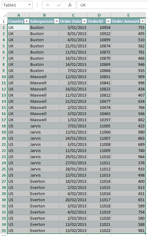
And I want the data for each salesperson on a separate sheet.
Tip: see the nice formatting of my source data? That is because I have inserted an Excel Table.
I’ve done this for a few reasons:
- When you insert a Table, Excel gives the table a name and structured references (you can see the Table name in the name box in the top left of the image above; Table1).
- When I insert my Pivot Table Excel will use the Table name as the source range.
- Then when I add new sales data to the bottom of the table it will automatically be included in my Table range. This means I don’t have to edit the data source of my Pivot Table to include the new rows of data. I can just click the refresh button and job done.
- If you don’t like the formatting simply select the Excel Table and from the Design tab select the Table Style ‘none’. It’s usually the first one in the list.
Structured references work in the same way as a dynamic named range except you don’t have to do all the work to set them up.
Click here for more on Structured References: see Magic Feature 4 in this Excel Tables tutorial.
Right, back to the task.
Inserting a Pivot Table
- Select any cell inside your source data.
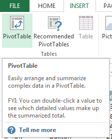
- On the Insert tab of the Ribbon select PivotTable:
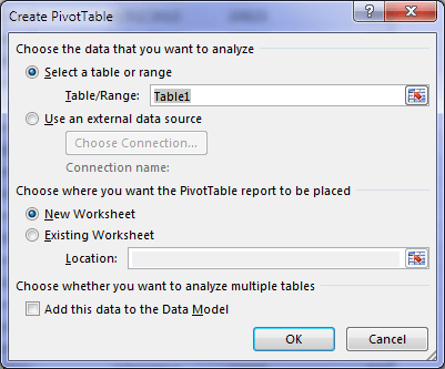
- Excel will automatically detect the range of cells and put it in your Table/Range field. Remember mine is called Table1. You can leave the default as New Worksheet and click ok.
- Ok, now you’re ready to build your choose the fields. We’re going to set up the first one for the sales person Buxton.
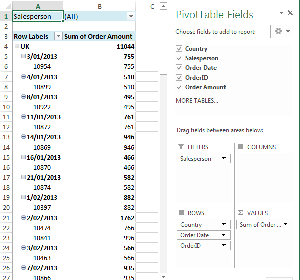
- drag the Salesperson field into the Filter area
- drag the Order Amount field into the Values area
- and the remaining fields go into the Rows area like this:
- Ok, so far so good. Let’s tidy it up now:
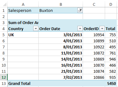
- Lastly, select the salesperson from the Filter at the top and now you’ve got your extract of the records for one salesperson:
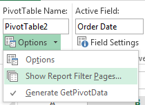
- Now to repeat the process for the other sales people, select the PivotTable then on the Ribbon tab PivotTable Analyze: Options select Options > Show Report Filter Pages....
Since we want every record listed (as opposed to summarising the data) we need to put every field in an area:
Note: if you don’t have a column/columns with amounts you can just drag all remaining fields into the Rows area.
Formatting
Select a cell in the PivotTable > on the Design tab under Report Layout select, ‘Show in Tabular Form’, and under Subtotals select 'Do not show subtotals'.
On the PivotTable Analyze tab deselect ‘Expand/collapse buttons’ as we don’t need these since every record will be displayed.
Tip 1: If you want you can turn off the Grand Total row. Right click the Pivot Table > PivotTable Options > Totals & Filters tab > uncheck ‘Show grand totals for columns’.
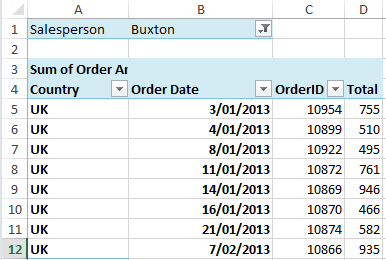
Tip 2: If you’ve got Excel 2010 or later you can repeat the country label down the column. Right click a cell in the Country column > Field Settings > Layout & Print tab > check the ‘Repeat Item labels’. So now it looks like this:
Excel will create a new worksheet for each salesperson in the filter.
Handling Blank Cells
If your source data has blank cells you might end up with the word ‘blank’ in your table like this in the OrderID column below:
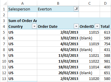
This is because each column (except the Total column) is actually a row label and it’s expected that the row labels will have a name, not be blank.
To remove the blanks simply click in one of the cells that contain the word ‘blank’ and enter a space in the cell. Excel will automatically replace all of the blanks with a space.
The good news is, if you later enter data in the source, the fields in your table will still bring this data in when you refresh the pivot table.
Want More?
How about automatically refreshing your PivotTables when you add new data.
Or, if you’re new to Pivot Tables check out this tutorial which will take you through the steps.
Extracting Data with Formulas
Before we had the FILTER function we would use convoluted array formulas that looked like this:
=IFERROR(INDEX(Data[#All],SMALL(IF(Salesperson="BUXTON",ROW(Order_Date),""),ROW(E1)),COLUMN()+2),"")
You had to manually copy the formula down to any new rows and if the inexperienced user forgot to enter it with CTRL+SHIFT+ENTER, it broke!
This approach was therefore error prone and fragile, which is why I always recommended using a PivotTable. However, now that we have the FILTER function we can easily extract data to separate sheets, and FILTER will automatically pick up new data as it gets added to the master sheet (assuming it’s formatted in an Excel Table). No need to edit the formula and therefore less chance of it breaking.
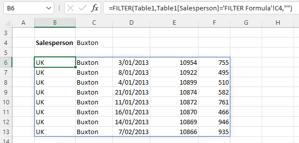
Using the example data in Table1 I can write FILTER like this:
=FILTER(Table1,Table1[Salesperson]='FILTER Formula'!C4,"")
Which returns the rows of data for the salesperson ‘Buxton’ selected from the data validation list in cell C4:
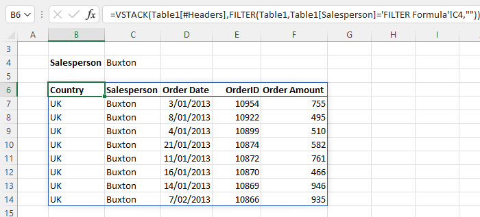
If you have Microsoft 365 you can improve on it by including the column labels using the VSTACK function like so:
=VSTACK(Table1[#Headers],FILTER(Table1,Table1[Salesperson]='FILTER Formula'!C4,""))
In the image below I’ve added bold formatting and a bottom cell border for the headers:
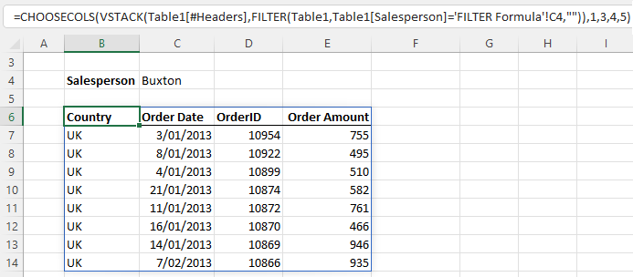
As already have the salesperson name in cell C4, we can exclude the salesperson column from the table using the CHOOSECOLS function (Microsoft 365 only):
=CHOOSECOLS(VSTACK(Table1[#Headers],FILTER(Table1,Table1[Salesperson]='FILTER Formula'!C4,"")),1,3,4,5)
Best Option for Extracting Data
If you don’t have the FILTER function, then by far the best option is to use PivotTables to extract data to separate sheets. However, if you have the FILTER function then I’d say there are pros and cons:
Pros and cons of using PivotTables to extract data:
- Pros: Easy to build, update and not easily broken.
- Cons: requires clicking on the Refresh button to get updates from the source table
Pros and cons of using the FILTER function to extract data:
- Pros: updates automatically
- Cons: More easily broken than PivotTables, more complex to write and if you're working with a lot of data, it could be slow to recalculate.

When I extract data from a large worksheet to individual worksheets, some of them have the correct tab name based on the filtered column text, but some have a number to identify the Btab rather than the text from the larger worksheet. This requires renaming the new worksheets to match the filtered column. What is the possible remedy for this?
Bill
Hi Bill,
That’s odd. Are there already tabs in the file with the name it should be? I wonder if it happens with name conflicts as I haven’t had that problem before.
Mynda
Hi Leanne, what a great video. A simple step by step guide paired with your amazing ability to walk the viewer through it. The evidence for Not all heroes wear capes.
Aw, thanks so much! Glad it was helpful.
Excellent article, Mynda. (No pun intended.) I am a fairly advanced Excel user, yet I never realized that pivot tables could spread the data across various sheets. My biggest frustration is that I seem to be on the tail end of the update curve, so I do not have access to many of the new functions in Excel 365 as yet, including CHOOSECOLS and VSTACK, so I can’t yet play with those. Regardless, I enjoy reading your tutorials. Keep up the good work!
Glad you liked it, Glenn! Sounds like you might be on the semi-annual update channel if you’ve already updated Excel and you don’t have these functions because they’re generally available to everyone on the current update channel.
Thank you so much for the tips and tricks!
I have a question.
I have created pivot tables and charts from a dataset. Is there a way to link these charts back to my dataset when I click on a chart component? For example from the chart, I would like to see a drill down of what that bar represents, I would click on the bar and it should show me event details of that category. Is this possible?
Thank you again!
Hi Amy,
No, Excel Pivot charts don’t have drill down functionality. Only the PivotTable itself. You could add buttons/hyperlinks above the chart that allows the user to navigate to an already drilled down view of the data.
Mynda
Hi,
This was really helpful, thank you!
I have a question.
I need to do be able to split sales persons sales onto separate tabs from a pivot table, but I need them to feed through to existing tabs, that have already been formatted and have specific formulas, to calculate commission etc.
Is this possible? Or can they only create new tabs with the pivot information?
Thanks in advance 🙂
Lucy
Hi Lucy,
The ‘Show Report Filter Pages’ option will only create new worksheets, but you can place the PivotTables on the sheets you want and then once they’re set up you just click the ‘Refresh All’ button on the Data tab of the ribbon.
Mynda
Hi
Dears,
please i’m looking for why my pivot table some times show the date column in the pivot ( split to 3 sections ) years , quarters and months.
not show the date as it write in the column.
thanks 🙂
This is the automatic grouping of date fields. You can CTRL+Z to undo it immediately after you add the field to the PivotTable, or you can right-click > Group > remove the groupings.
thanks a lot for your support
and really you are amazing about sharing the information with the others.
thanks,
Mynda
You’re welcome, glad we can help.
regards
Phil
This was very useful and interesting. Thanks.
Thanks for sharing a blog on excel pivot table. This will help to extract your data easily. If you want to enhance your skills in Pivot Table then you can join advance excel course
It’s great to know we could help, Kritesh 🙂
When I follow these steps, I get a large box to the right (the drop fields box, I think). How can I get rid of it? My users think it is ugly and I have to agree, but when I try to delete it, excel won’t let me.
Thanks. Great tutorial, easy to understand and to implement.
Hi Carol,
If you refer to the Field List shown on the right side of the sheet when you click inside a pivot table, you can hide it by simply right clicking on any cell from the pivot table and choose “Hide Field List”. If it’s hidden, you can display it back in the same way, choosing “Show Field List” from the right click menu.
Cheers,
Catalin
I see,
But I think Excel provided lots of logical formula so it must be a way that if some of formulas combine all together the result can be come out.
Hi Dritan,
You can use formulas to do just about anything in Excel, but that doesn’t mean they’re always the best way to ‘skin the Excel cat’ so to speak. For what you want to do this is by far the best, most efficient and robust solution. Just give it a go and you’ll see how easy it is.
Kind regards,
Mynda
Hi Mynda,
I thank you for your advice, I have learn lot from your training.
You’re excellent in Excel.
Kind regards,
Dritan
You’re welcome, Dritan 🙂
Hello Mynda,
I’m new to all this Excel Hubbub, but I have to say – I quite agree with all of the testimonials I read in your favor. Those were supportive of my continuing to look into your material. However, when I downloaded this workbook sample, and stepped through your instructions, the light bulbs kept popping. Now, I can’t wait until I can get enough of your course material digested to get to the dashboard training. Would love to do it now, but even at a discount I think I’d be in over my head. I am grateful to benefit from your early frustrations and tranformational evolution.
Cheers!
Bud
Hi Bud,
Thanks for your kind words. I’m glad you’re enjoying out tutorials and they’re helping you get your head around some of the techniques 🙂
Hope to see you in the Dashboard class some day.
Kind regards,
Mynda.
I’m pretty sure I posted a comment the other day but maybe something went wrong. Anyway, I don’t think the following is the case in Excel 2007/2010:
“This is because every time you insert a new PivotTable Excel creates a copy of the source data, called the Pivot Cache, …”
From my experience Excel uses the same cache by default although I do remember the behavior you describe from 2003 though.
Hi m-b,
Thanks for sharing. I didn’t see your previous comment, sorry about that.
I did a bit of research and you’re spot on. This is what I found:
“Excel automatically shares the PivotTable data cache between two or more PivotTable reports that are based on the same cell range or data connection. If the cell range or data connection for two or more PivotTable reports is different, the data cache cannot be shared between those reports.”
Read more about the Excel Pivot Table cache.
Cheers,
Mynda.
Hello Mynda,
In this situation with Excel 2010 couldn’t you keep all of the Salespersons selected in the Report Filter and after you have the pivot table formatted with Country, Order Date and Order Id go to PivotTable Tools Option tab and click on Options under the PivotTable Name: and select Show Report Filter Pages. Then click on Salesperson and each Salesperson is copied to its own worksheet tab. I find this quick and easy.
Yes, Theresa, that’s a great, quick way to achive the same result. Thanks for sharing 🙂
Hi Mynda
Great website and tutorials. Easy to understand.
The show report filter option is great to create the separate pages. In my case I want to run a report for departments showing staff wages from a master sheet of all staff and wages. If I want to email the individual page to a manager, all of the data is still there and by using the filter options, data from other departments can be displayed. Is there a way of sending the separate page created and removing the filter options so that the manager just receives the data for his or her own department?
Kind regards
Leanne
Hi Leanne,
Thanks for your kind words. I’m glad we can help.
To answer your question; there’s no way to automatically restrict access to the soucre data or filter options. The only thing you can do is copy the individual worksheet containing the PivotTable to a new workbook (without a link to the original file), for distributing to each manager. Make sure you either copy and paste as values or break the links to the original file.
If you know VBA then you could write some code to automate this.
Kind regards,
Mynda
Hi Mynda
Thanks so much for the prompt reply. I tried to copy to a new workbook by copying and pasting as values which worked thankyou. You also mentioned that I could copy and break the links to the original file. Is that another option – I am not sure how to do that.
Kind regards
Leanne
Hi Leanne,
I wouldn’t worry. It’s quick just to copy and paste as values with formatting.
Mynda
Thanks Mynda.
Hi Leanne,
Try this tutorial:
excel-pivottable-expand-collapse-show-details
Pay attention to the “Show Details” section.
If you select and filter for a department, and double click on the Totals cell (or right click and choose “Show Details”), a new sheet will be created, and it will contain only a defined table with data for that department.
Cheers,
Catalin
Note: What Catalin is describing will show all of the transactions for the department, as opposed to the summarised data for one department.
Either way you need to copy the worksheet into another workbook.
Mynda
Thanks Catalin for your prompt reply. I tried as you suggested and that worked also. I will have to have a play now and work out what will be the best method.
Kind regards
Leanne
You’re welcome Leanne 🙂
Catalin