I'm about to show you how one overlooked tool can transform the way you work with data. It's not a complex formula or a hidden setting - it's something so fundamental you'll be shocked you haven't been using it all along. Of course, I'm talking about Excel Tables.
Before you say, "Oh, I know all about Tables," wait because I might just show you something you didn't know. And if you aren't familiar with Tables, after reading this you'll kick yourself for not using them sooner.
And if you are one of the few who have been using Excel Tables, share your favourite tip in the comments.
Table of Contents
- Excel Tables Video
- Get the Practice File
- Creating a Table
- Table Features
- Table Styles
- Freeze Panes vs Pinned Headers
- Filters
- Structured References
- Referencing Tables in Formulas
- Absolute and Relative Table References
- Automatically Update Reports
- Slicers
- Total Rows
- Automate Your Workflow with Power Query
- Next Steps
Watch the Excel Tables Video

Get the Practice File
Try tables yourself with the practice file:
Enter your email address below to download the sample workbook.

Creating a Table
Excel Tables work great with data both big and small. You might have heard a rumour that tables over 500 thousand rows can slow down your file, but you'll be pleased to know that this issue was fixed in Excel 2016 and is no longer a problem.
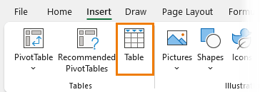
To create a table, select your data and press `CTRL+T`. If you can't remember the shortcut, you'll also find the option on the Insert tab under Table:
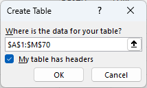
If your table doesn't have column headers, you can uncheck the box in the Create Table dialog box:
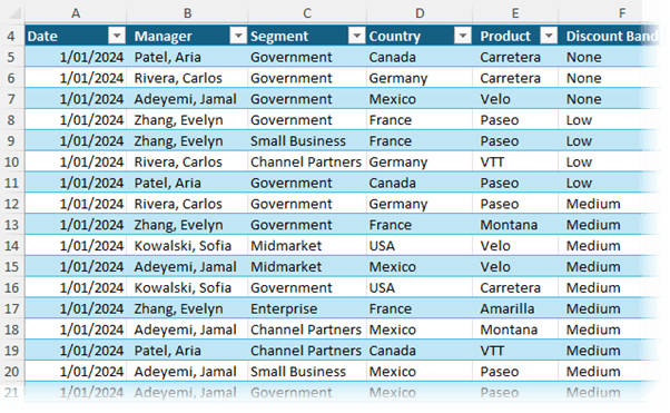
Instantly, Excel formats your data and adds filter buttons to each column header:
But that's not all - let's step through the features.
Table Features
With a cell in the table selected, you'll see a contextual Table Design tab on the Ribbon. Here, in the far left you can rename your table from the default name (like Table1) to something more useful, such as SalesData. This becomes important as you work with your table data.
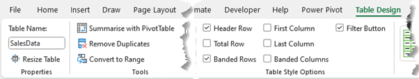
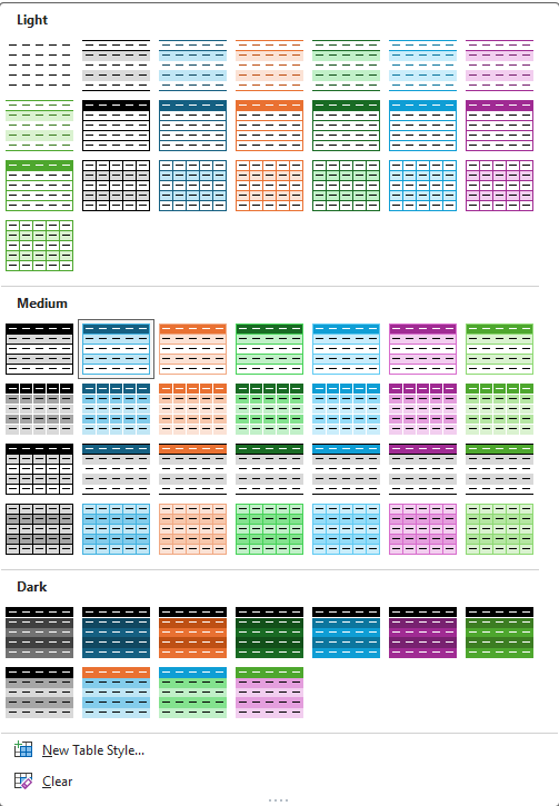
Table Styles
The most noticeable feature of tables is the banded row formatting, allowing your eye to easily scan across the columns while maintaining focus on the desired row. This not only saves time but also helps reduce errors when editing and entering data.
If you don't have wide tables or need more subtle formatting, you can choose from different formats in the style gallery, including the 'light' style or create your own custom style.
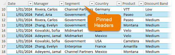
Freeze Panes vs Pinned Headers
When working with large tables, you might often resort to freezing panes to pin the headers as you scroll down. However, with Tables, the headers automatically stay visible when you scroll, even if they don't start in the first row.
Filters
The filter buttons added to each column header are significant time-savers. With just a click, you can sort and filter your data to find exactly what you need in seconds.
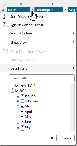
Filters make it simple to narrow down your data to the most relevant information without manually searching through rows and columns.
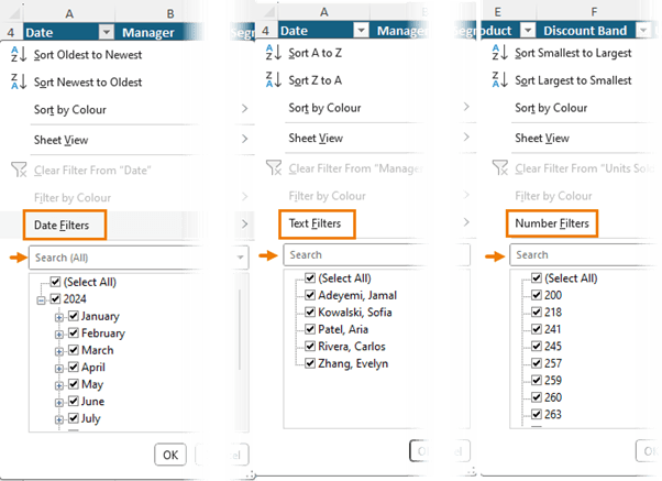
You'll have different filter options depending on the type of data in the column, and you can even use the search feature within the filter drop-down:
Structured References and Dynamic Ranges
Adding calculated columns is one of the most common tasks you'll perform when working with data. For example, in my dataset I have columns for sales and cost of goods sold (COGS) but no column for Gross Profit.
Inserting a column header in the first empty column to the right of the table will result in the table automatically expanding to include this new column in the table range.
The formula for Gross Profit is (Sales - COGS) and when you insert this in a table is uses the table's structured references instead of regular cell references. Structured references consist of the column name prefixed by the @ symbol, which tells Excel to refer to the cell on the current row. When you press ENTER, the formula is copied down the remaining cells in the table:
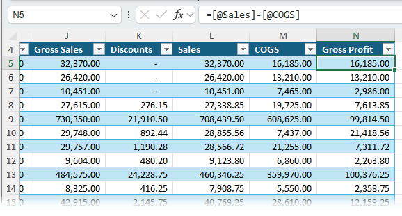
Not only is having the same formula in a column best practice, but it also makes it easy to understand what the formula is calculating because the structured references display the column names.
Referencing Tables in Formulas
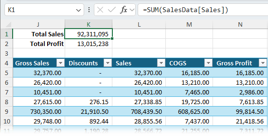
You can also reference tables in formulas from outside the table. For example, to get some headline figures like Total Sales, you can use your mouse to click in the column header and select the Sales column.
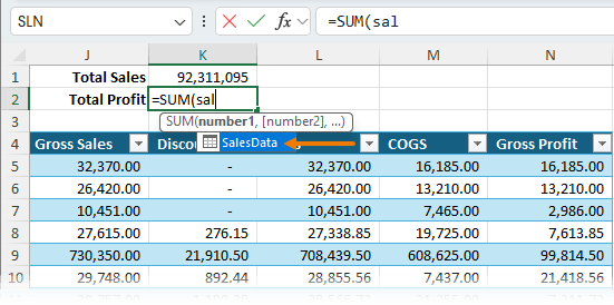
You can also use IntelliSense to write formulas. For example, to calculate Total Profit, you can type in the table name, and Excel will auto-complete it for you:
Then to insert the column, type an opening square bracket:
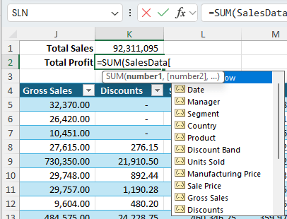
Use the arrow keys to move through the list or type in the start of the column name to narrow down the options. Tab to insert the column name.
You can also reference the table with its structured references from any sheet in the workbook, making it easy to write and understand formulas.
Not only are formulas that use the table's structured reference quick and easy to write, they're also easy to understand what and how the formula is calculating. Plus, they automatically update when new data is added to the table, so you never have to edit cell ranges in formulas again!
Absolute and Relative Table References
Unfortunately, you can't use the F4 key to apply absolute references to Structured References in formulas. They have some quirky rules depending on whether you're copying and pasting a formula or left-clicking and dragging it. You'll find more on working with absolute references for Table Structured References here.
Automatically Update Reports
If you create any type of report that gets updated regularly, the most time-consuming task is editing the formulas, PivotTables, and charts to include the new data. But when you format your data in a Table, you don't have to do this repetitive and laborious work.
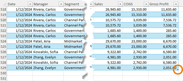
For example, if your source data table has data up to November, and you receive new data for December, you can simply copy and paste the December data into the next blank row below the table:
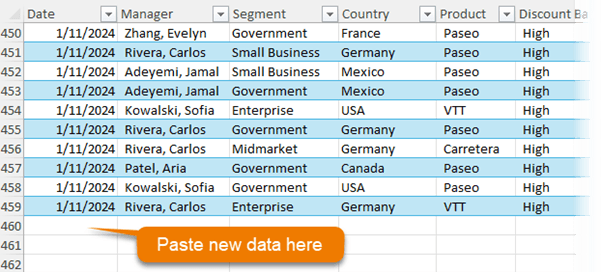
The formatting and formulas will automatically update to include the new data. We can see below the table range pull handle is now in the last cell of the December data:
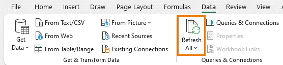
To update your report, go to the Data tab and click Refresh All:
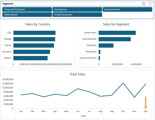
With one click, all your PivotTables and charts will include the new data:
Slicers
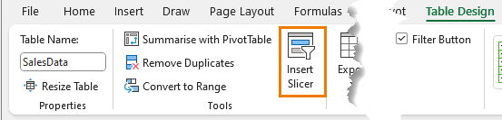
You might be familiar with Slicers from PivotTables, which make filtering your reports super easy. But did you know you can also use Slicers with Tables? Select a cell in the table, then on the Table Design tab, click Slicer:
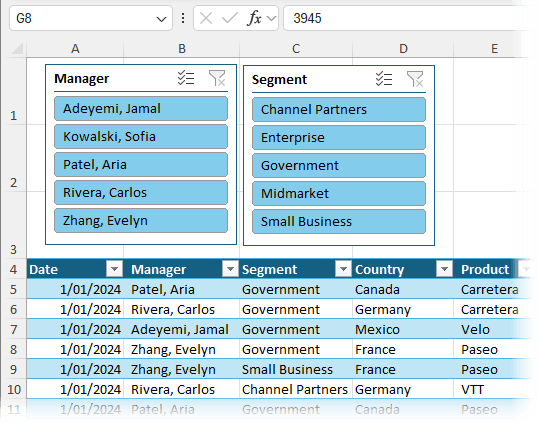
Choose the columns you want slicers for, and you can resize and position them as needed.
Slicers make it easy to focus on the data you're interested in and visually indicate what items are included in the table.
Total Rows
Another built-in feature of Tables is total rows. You can turn them on in the Table Design tab by checking the Total Row box:
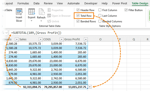
It automatically adds a total to the last numeric column, but you can add totals to other numeric columns by clicking the drop down list button and choosing the aggregation type.
The nice thing about these totals is that they use the SUBTOTAL function, which excludes rows hidden by filters.
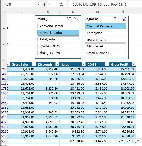
As you select different items in the Slicers, the total row automatically updates accordingly:
By integrating Excel Tables into your workflow, you can significantly streamline your data management tasks, making your processes more efficient and less error-prone. Give it a try, and you'll see just how transformative this overlooked tool can be.
Automate Your Workflow with Power Query
Above, I showed you how to update tables by pasting in your new data. If you want to learn how to automate this process, including merging multiple files in seconds and transforming messy data into Tables effortlessly, check out my tutorial on How to Easily Automate Boring Excel Tasks with Power Query.
It will show you how to save hours on data preparation, making you the go-to Excel guru in your office.
Next Steps
We've just covered a few of Excel's powerful features. But there's much more to discover.
If you've found this information valuable, you'll be interested to know that my Excel courses dive even deeper. Including everything from advanced formulas to advanced data analysis techniques designed to significantly enhance your Excel proficiency. Click here to check out our complete Excel Course library.


Hi Mynda, I really appreciate your work, and I am learning a lot from you. So many thanks!
A question: using MS Excel 365, I am trying to use tables with the notation table[field], defining names for tables.
They can be used in every Worksheet, and this is great.
Is it possible, though, to use in different workbooks?
For example, I have a workbook A for invoice data (where I defined tables with names), and a separate workbook B to do some other calculations, and I’d like (from B) to address the tables in Workbook A, but it doesn’t seem possible. How could it be done?
I’ve tried also with Power Query, creating (in Workbook B) a connection to Workbook A, but again, it seems that named tables are not visible. The only way I found – pretty primitive – is to COPY (via Power Query) the whole data…. Is there a simpler (or better) way?
Thanks again
Giuseppe
Hi Giuseppe,
Use your mouse to select the table column in the external file and Excel will insert the correct reference for you that includes the file name. Or use Power Query to Get Data > From File > From Excel and follow the prompts to browse to the file. Note: the file needs to be closed for Power Query to reference it.
Mynda
Thanks Mynda, I’ve tried.
Second method (Get Data) successful –> it creates a new sheet in my file B with a dynamic copy of the table with the same name, so I can address the tablename[field1], tablename[field2], etc.,
Which is fine for my purposes… The only disadvantage is that I have several new sheets in my Workbook B (one for every table I get data from Workbook A). Is there a way to get the same result WITHOUT adding new sheets in my workbook B?
I couldn’t succeed very well, though, in the first method….. So please let me understand better. My steps are: in my workbook A (where I defined tables with names, i.e. tablename[field1], tablename[field2], etc.), I use mouse to select the table column (downward arrow). OK, selected and copy it.
Now, in my Workbook B, I paste the selection:
1) using “Paste Special” with reference/link, I get the data of the whole column as links of the specific cells of my column (let’s say in cells A1, A2, A3, and so on) in the format =[filenameA.xlsx]!A1 –> Which is not what I would get (I cannot use them as fields in a table).
2) using “Insert copied cells” I get the whole data of my column, but I have “only” the values of the cells… not the link….
Sorry, maybe I’m missing something ….. Could you please explain me a little bit more?
Thanks again for your support!
G
Hi Giuseppe,
I think it’s time for a Power Query course. It’s difficult to teach you here in the comments, however I’ll try to give you some pointers:
Power Query – once you connect Power Query to data in Workbook A and load the data in Workbook B, to get updates from workbook A, you simply right-click on the query table in Workbook B > Refresh. No need to create another query unless you have a new table in Workbook A that you want to also bring data in from. However, even if you have multiple tables in Workbook A, you can consolidate them into a single table in Power Query and load the data into Workbook B. More on this in my Power Query course.
To link formulas to tables in external workbooks: start your formula in Workbook B e.g. =SUM( then use your mouse to navigate to workbook A and select the table ranges you want to reference in the formula with your mouse. No copying and pasting, just references. By using your mouse here, Excel will automatically insert the full table reference including the file name.
If you’re still stuck, please post your question on our Excel forum where you can also upload a sample file and we can help you further.
Mynda
Great Mynda, I followed your tip and now it works!!!
Yes, I’m seriously considering to attend your Power Query course in the near future… So to explore all the great functionalities it offers.
Thanks again for your quick answer (and your patience, too!).
G
Great to hear!
Table total rows are great. But they can be even better.
When the Table total cell has focus it displays a drop down arrow beside it. Click on the arrow and it shows a list of 8 functions, including sum.
Average, Count, Count Numbers, Max, Min, Sum, StDev, Var, More functions …
Cheers, Ron! I demoed that in the video at 10:14 but forgot to show it in the screenshot in the post above. Thanks for mentioning.
Hi. Always like getting your newsletter – almost always find something I didn’t know. (not suprising as I am still’novice’). The 30 June issue deals with tables. I have a bit of an issue with one I created. Lots of cells full of text. I have named cells (named in the ‘basic’ way) using the Name Box. If I add a new line at the bottom of the table and then sort this into order the cell name don’t go with the data so that if I click a hyperlink on another sheet to take to specific data it goes to the wrong place. Do I need to master Structure Referencing — will that resolve this issue. Currently I just have to remember to use Insert to enter new data in the ‘correct place.
Thanks for all the assistance.
Regards.
Hi Barry, if you need the name to move with the cell as it’s sorted, then you’d need to write a dynamic named range. https://www.myonlinetraininghub.com/excel-dynamic-named-ranges
Which lesson would I need for:
I need a table to Pop up when I click into it
Nothing fancy – just a 15 rows by 5 columns
Clarification to above – I need a pop up table to “pop up” when I click into a specific cell.
Because you want to enter data into it, or just containing information? Please post your question on our Excel forum where you can also upload a sample file and we can help you further.
I’ve created a personal checkbook and love that it is in a tabular format so that I can quickly look at spending in various categories or months by filtering the columns but I have the issue of maintaining a running balance. You take the previous rows balance then add the credit and subtract the debit of the current row. I wrote a macro that I have to run every time I add new entries. Is there a better workaround?
Respectfully,
Bob Marolt
Hi Bob,
Please see this tutorial: Excel Table running total formula.
Mynda
Hi
Madam Philip Treacy
Kindly teach me formula of auto schedule of semi annual dates of 5 years
for example 2 installment in each date of 01-01-16, 01-07-16, 01-01-17, 01-07-17, ……..01-07-20
if i put only 5 year, 2 installment, the formula auto set schedule of each semi installment of future date till last installment date
Regards
Salim Gul
Hi Salim,
It depends on which version of Excel you’re using. Please post your question on our Excel forum where you can upload a sample file showing your data and what you’d like to see. Also let us know your Excel version.
Mynda
Great information; what I have found giving excel classes etc is that many folks don’t know that tables can have slicers. You don’t need a pivot table to have slicers, they work with ranges converted into tables.
Thanks Richard
ITS A EXCELLENT TUTORIAL-MANY MANYTHANKS
You’re welcome.
I’m a big fan of Excel tables and their structured referencing. Much more intuitive than R1C1 style addressing when referencing table rows and columns.
But one thing I *dislike* about structured referencing is that, when I copy a formula from one table column to another, and the source column includes a structured reference to another column, that reference doesn’t change in the target column as it would with relative references.
For example, suppose I have a table containing month columns (Jan, Feb, … Dec), and the Jun column contains the formula =1.1*[@May]. If I copy that formula to the Jul column, I end up with the same formula (=1.1*[@May]), not =1.1*[@Jun] as I might expect.
That’s because structured references are, by definition, absolute. If relative references are desired in a table, they must be the standard R1C1 style addresses.
I wish Excel provided a way to tag a structured address as relative, similar to how I can use $ within an R1C1 style address to tag a row or column as absolute. I could then copy formulas from one table column to another with the expected (relative reference) result.
Hi Paul,
Strange, by default, table structured references are relative, not absolute, the column name should change when you copy the cell to the right.
You can make structured references absolute, here is a tutorial: excel-table-absolute-structured-references
If you want to prevent the formula to change the column name when the formula is copied across, the absolute reference should look like this:
=1.1*Table1[@[May]:[May]]
Catalin
Sure doesn’t work that way for me. When I *copy* a formula from a table column containing a structured reference to another table column, the column name reference *does not change*. That means, at least in the case of copying/pasting, structured references are absolute, not relative.
Apparently, as I just discovered, if you use a cell’s handle to drag it’s formula to another cell, any structured references in the formula *is* treated as relative, and changes accordingly in the target cell.
That’s wildly inconsistent. R1C1 type references certainly don’t behave that way: if a cell’s formula includes a relative R1C1 address (no $ prefixing the row and/or column), copying or dragging that cell to another cell produces the exact same result. Why shouldn’t structured references behave the same way?
In my opinion MS made a mistake here. Structured references *should* be relative by default, just as R1C1 style addresses are relative by default, and should produce the same result whether the cell is copied or dragged.
Hi Paul,
There is indeed a difference between copying and dragging a cell with a formula in a table, but it’s not the only difference between normal excel cell references and structured references. For example, there is no switch to make the reference absolute in a table, like the $ sign in a normal cell reference.
Can’t tell if this is a mistake or not, a table is a complex object, it’s hard to transfer all normal operations to a different type of object.
Just knowing these differences, should be enough for you to decide what operation you should do, right? 🙂
Catalin
Love the column chart… Like to know how you combined the 3 columns (Data, Max, Min) into one for the chart. Also how did you get the column color and only the correct data label to follow – did you use Conditional formatting?
FYI – I did add different numbers to the data and the column (line chart did also) came out correctly.
If you do not have time to reply, I understand but these are something that would be very good in the classroom and in business.
Hi Burdette,
For the benefit of others reading this, your question is referring to the charts on this post: https://www.myonlinetraininghub.com/label-excel-chart-min-and-max
The Data, Min and Max columns are set to overlap as per step 3: Overlap columns; right-click any column > format data series > Series overlap 100%, Gap width 60% (or whatever you prefer).
The colors are set at the series level as per step 4: Colour code min/max; left click the max column > format the fill colour. Repeat for the min column.
Kind regards,
Mynda
Excellent explanation
Thanks, Arif 🙂
Hi Mynda,
I am trying to create a structured reference using this formula – “=LEFT(C2, LEN(C2) – 3)”. Please could you help me with this?
Table name = P01table
Column specifier = name
Item specifier = #Data
Thanks a ton!
Hi Akhil,
If you type this formula in the same table in another column, excel intellisense should automatically enter the table reference if you select a cell from the table
=LEFT([@name], LEN([@name]) -3) should be the formula.
If the autocomplete feature does not work, check your settings from File-Options-Formulas-make sure the option: Use table name in formulas is checked.
Hi Catalin,
Thanks so much for your help – that worked absolutely perfectly!
You’re welcome 🙂
Hi Mynda,
This seems like a simple problem, but I’m struggling. Maybe you can help.
I’m using a userform for data entry, with a listbox tied to a named range (MainDB). When I add a new record, I can see the database update, but the list does not update properly until I exit the form and return. Is there a way to refresh the listbox data without exiting? Should I convert the named range to a table?
Thanks for any help you can provide.
Bill
Hi Bill,
Usually, that listbox is populated when the form is activated. If you add new values to the source of the list, you should write code to update that listbox (use a new procedure to update list: clear existing entries and use the same code you have for populating the listbox again)
To clear the listbox: listBox1.Items.Clear()
Catalin
Excel Tables are 1 of those fabulous features, I use them almost invariably now.
Nevertheless, there is 1 thing that one should bear in mind. Before setting up an ET or converting an existing data set to an ET, one should carefully consider the following.
When a new row of data is added to the ET, the AutoComplete is done based on what is in the 1st row of data. If, after setting up an ET one wants to add a new row to act as row 1, hoping to have that new row update existing rows & fill in new rows at the bottom, it won’t work, i.e. it does not update.
One could convert the ET back to a normal table, then reconvert into an ET, but that only sometimes do the trick. I have not come across a satisfactory solution for this.
In my opinion the best way is to carefully plan beforehand what data should be in row 1, then stick with that.
Indeed, Peter. Tables are designed with consistency in mind. Therefore the formula in row 1 should be the same for the entire column.
Mynda
checking it out now
I’ve recently found your site and guidance; they’re excellent and very informative. Congratulations.
I have a question about remote access to Excel Tables. I’m using MS Office Professional Plus 2013.
In one workbook I have a number of data tables (the Source). Some of these have been formatted as Excel Tables, some as named ranges.
A separate workbook has been configured as an Excel Template from which I generate a number of different workbooks that look up data from the Source dependent on a drop-down constrained list. The setup works really well and the newly generated workbooks populate properly and update when the Source is changed and when they are opened or forced to refresh data.
EXCEPT I’ve just discovered that the data is not looked up if the Source is not open. Look ups to the named ranges work whether or not the Source is open. Look ups to the Excel Tables do not. If I have a generated workbook open when the Source is closed the looked-up cells are blank (due to IFERROR). As soon as I open the Source, the blank cells populate properly and immediately.
Is this something that is known or designed, or do I need to start error tracking? I’m using Excel Tables because the data in the Source is dynamic. If I can’t use Tables I suppose I’ll have to go back to OFFSET.
Thanks for your help.
Stephen
Hi Stephen,
Welcome to MyOnlineTrainingHub, glad to hear you like our materials.
What “Lookups” are you using? VLOOKUP or INDEX-MATCH?
I would extract data from the Template with Power Query, this way you will no longer have external links, and you will still be able to refresh data from Template. It’s a much stronger setup, in my opinion.
Cheers,
Catalin
Hi Catalin,
Thanks for your reply. I’ve done some more work on this since I posted and I’ve established that the remote lookups (using INDEX in an Array formula to return multiple matches) do not work when the source is an Excel Table, unless the source file and the destination file are both open on the same computer. The same formulae work when the source is a Named Range, even if the source is not open, and even though the cell references for the Range are identical with the Table. I find that very odd.
I should mention that this is on a corporate infrastructure so clients using the documents might be in different parts of the UK, and all the files are on a central SharePoint server. I don’t think the Excel has Power Query installed and I can’t add it to the corporate installation.
I’m managing the central source index and I can do most of the reporting on my local machine, my issue was just making sure that any time anyone opened one of the destination documents it always contained the current data, looked up as it opened. I’ve achieved that by eliminating Tables, I just have to manage the changes in range myself. When I get time I’ll automate that as well!
Thanks for your help.
Stephen
Then you can try to bring source data from Data tab, Get External Data section, From Other Sources – From Microsoft Query , from excel files. You will have to browse to your excel file, then select the tables/sheets you want to bring into your file. This data connection is refreshable also.
Cheers,
Catalin
This would be great as a video!
So well presented–concise and so easy to read…passing on to my staff. Thanks.
Thanks, Gord! Glad you found it helpful.
Hi Mynda,
Is there option to sub total in Excel table
Hi Kamran,
No, you can’t use the Subtotal tool in an Excel Table, but you can use a PivotTable to summarise and subtotal the data.
Mynda
One other nice feature to mention is that when you scroll down a table to the point where the column headers would normally disappear, those headers get “absorbed” in the column in place of the column’s letter designation. That way you don’t actually have to freeze your headers in a long table.
I am not able to download: Excel_Blog_Workbooks.xlsx (https://www.myonlinetraininghub.com/wp-content/moth-practice-files/Excel_Blog_Workbooks.xlsx).
Hi Carl, try to right click the link and choose: Save link as or Save target as, depending on your browser. Make sure it is saved as xlsx, your browser might change the extension.
Cheers,
Catalin
Hi Mynda,
I have a Table (Table1) in columns B thru H
I have this formula in K5 =J5+Table1[@Days]
I want to fill across from K5 to BD5
I want J5 to increase as I go (J6, J7 etc) but I want the table reference to stay absolute.
I can do this one cell at a time by selecting K5, then hitting Ctrl+R, L5, then hit Ctrl+R etc
But I can’t seem to do all the cells with a single swish
Can we make table references absolute?
Regards – Dave
Hi Dave,
You have to duplicate the column name, to make it absolute:
=Table1[@[Days]:[Days]]
You will find more info here: excel-table-absolute-structured-references
Catalin
Ah, OK, thanks. To create the original formula, I typed ‘J5+’ then clicked on a cell in the table. Is there some way the absolute table reference can be entered by clicking, or do I have to type it in manually?
Dave
Unfortunately, yes, you have to type it manually, there is no shortcut for this.
Catalin
Ok Catalin, thanks for your help.
Thanks for the information. Well done.
However it’s a pity that you don’t describe how to turn off Microsoft’s ridiculous idea of automatically naming columns column1, column2 etc.
It would also help if you explained how to use Table Formula Shortcuts, such as Table1[#All] or one column =Table1[[#Headers],[Column1]]
Hi Rob,
The automatic naming is not optional, it cannot be turned off. Power Query and Power Pivot will also give automatic names to new columns if you don’t provide one, excel cannot work with columns with no names…
The Table Formula Shortcuts should be used like any other range reference in a formula, they are structured references to excel ranges.
For example, if the range A1:C10 contains an excel table, where row 1 is the Headers row (with these column Names: Agent Name, Month, Sales), and you want to sum the data from column C, a formula will look like this: =SUM(C2:C10)
With structured references, the formula will look like this: =SUM(Table1[Sales]). Structured referfences will make formulas more readable, because you can actually understand what the formula will sum, without the need to go to the range of cells C2:C10 to see what is in those cells.
Note that you refered to a table column like “one column =Table1[[#Headers],[Column1]]”. The expression is refering to a single cell, in headers row, column 1, not to the entire column 1. A reference to a column will look like Table1[Column1], or Table1[[#All],[Column1] (this last expression includes the column name, not only the data range)
Cheers,
Catalin
This is not new nowadays however like it as easy to share and coach my colleagues. Thanks
Cheers, Le.
You’d be surprised how many people haven’t heard of Excel Tables. Microsoft esimate only 1% of Excel users know of and use Excel Tables!
Spread the word 🙂
Mynda
Hey Mynda,
I put the formula in as above BUT this is what it looks like on my sheet
=[@Salary]/Table9[[#Totals],[Salary]]
WHY would that be?
Thanks
Hi Justine,
In Excel 2010 the way you reference a row changed to =[@row], whereas in Excel 2007 it is =Table1[[#This Row],[Column1]].
I’ve updated the post above to include this update.
Kind regards,
Mynda
Download the workbook and practice what you learn. (https://www.myonlinetraininghub.com/wp-content/moth-practice-files/Excel_Blog_Workbooks.xlsx) is not working.
Unable to download
Hemant,
I tested it and it works for me. It may be your browswer. Please rignt-click the link > Save As > choose your folder you want to save it in. Make sure the file extension is .xlsx
Let me know if you’re still having problems.
Kind regards,
Mynda
Thank you very much , now everything starts to make sense in my brain…;)
Glad we could help, Faridz 🙂
thank you! I have read up on tables since I watched you Dashboard training a few weeks ago, but this was a great summary!
Thanks, Lindsey. Glad you’re making use of Tables 🙂
I am working with the instructions above however i cannot understand the comment “Tip: Format the cell before you enter your formula. in Excel Table Magic feature #3. can you help please?
Hi Martin,
Point #3 explains that when you enter the formula and you will see that the table automatically copies the new formula and formatting down the whole column to the bottom of the table. This is known as AutoComplete.
I hope that clarifies things. It doesn’t really matter if you format before or after entering your formula but I find it’s quicker to select one cell to format than a range of cells that might expand past the visible page. I prefer not to format entire columns as it can bloat your file size.
Kind regards,
Mynda
Seriously. Before finding your site, I had considered myself a bit of an Excel guru. Now, I feel like I don’t even know a fraction of what there is to know about Excel. Fortunately, because of my background, your webinars & tutorials are very easy to follow and apply immediately. Working in Process Improvements and Change Management, I can use the new features I am learning about on a daily basis to inform leadership and monitor our progress.
Thank you!!!!
Thanks, Miffy. I’m glad you’re enjoying our site and finding loads of useful tips.
Mynda
Hi Mynda,
This tutorial is excellent and fulfills all the required information that is necessary for the creation of tables and insertion of Data along with Formulas. I really admire your endeavoring that are helpful people like me and I am really thankful and grateful for your kindness with respect to spreading knowledge.
Always stay blessed.
Thanks, Tayyab. I’m glad you found this tutorial helpful 🙂
Hi Mynda,
Magic Feature #3 is not working for me when I download your practice sheet. Is it possible it is because I am using Excel 2013? I had to manually add the new column to my table. When I added the formula, I had to right click on the cell to get the option to copy down.
Second question on the extra column, I created a % of total by writing the formula: =[@Salary]/table1[[#Totals],[Salary]]. However, if I want to change the total line to maximum then the formula changes to % of maximum. Is there an easy way to keep it constant even if I change the way I look at the total?
Hi Suzanne,
Magic Feature #3 should work in Excel 2013. The trick is to put the formula in the very next available column. If you skip a column Excel will not include it in the table.
To fix your % of total change your formula to this:
=[@Salary]/SUM([Salary])
Kind regards,
Mynda
Or =[@Salary]/SUBTOTAL(9,[Salary]) if you want the % to just be of the rows that are visible (like when you filter the table).
Though looking at the date of this thread you’ve probably figured that out by now 🙂
Hi Mynda,
This is just a thank you note.
I have been exposed to your emails since I took Dashboard webinar.
The webinar as well as the emails are very clear and helpful.
All the best
Moshe
Thank you, Moshe 🙂
I’m glad you’re finding our training helpful.
I do Excel development using a lot of VBA and while I only use tabular data (thought you’d appreciate that) I’ve not formally used Tables before. I have an upcoming project where they might be appropriate but it was not clear from the article if or how to reference the Table data using VBA.
Could you comment on that or point me in an appropriate direction to get more information
Some great material on your web site, clear and easy to understand.
Thanks
Brain
Hi Brian,
The syntax to refer to table objects is quite simple:
-To refer to an entire table:
Range(“TableName”)
-To refer to a column:
Range(“TableName[ColumnName]”)
-To refer to Headers:
Range(“TableName[#Headers]”)
To easier manipulate the table, you can refer to table components , using ListObjects method:
Sheets(“Sheet1”).ListObjects(“TableName”).HeaderRowRange is identical to Range(“TableName[#Headers]”)
More info you can find at:
the-vba-guide-to-listobject-excel-tables
Cheers,
Catalin
Hello Mynda,
I take your dashboard online course. I do follow the links you put to understand better the subject. Here it says download the data but it doesn’t work. I wonder I do some mistakes? I have mac 2011 excel.
Thank you for respond in advance
Ozen
Hi Ozen,
I suspect your PC/Browser is changing the file extension when you download it. The file is a .xlsx file so please ensure when you right-click then File Save As that the file extension is .xlsx and if not please change it. You should then be able to open the file like any other Excel file.
Please let me know if you still have problems.
Mynda
Hi Mynda,
I really really appreciate your messages and my words are insufficient to explain my thanks. I thank you many many times.
I will tell you how I solved the issue. My problem was with the link (Download the workbook and practice what you learn) on above the page. When I tried to download the link I was getting a page with written an ascii code. It was not an excel file. So I copied the link in an excel worksheet and then I tried to open the link. Yay! Here the excel file is. It works well.
My macbook might cause the problem, I don’t know what the reason was. Anyway it works well and I am on my way to learn from your excel pages.
Thanks again for this great job you do.
Hi Ozen,
It sounds like you were originally left-clicking (or the equivalent on the Mac) the link and your browser was trying to open the Excel file. Whereas you should be right-clicking the link and saving the file as an Excel file and then browsing to the file location to open it.
Not to worry. The main thing is you have managed to open it.
Kind regards,
Mynda
Mynda
This was great! I had Excel for Mac 2008 at home for several years while I was working with Excel 2007 in Windows at work. Have since upgraded to Excel 2011 at home. Am slowed down a bit by having to “translate” concepts between the platforms, but it was very helpful to learn about Excel tables. In particular, I want to incorporate Structured References into my current project.
And those Magical Features – they ARE just that! It might be nice to see these illustrated in a future video.
What’s been most helpful is to be able to listen to your Dashboard tutorial, stopping every few slides to read your related tutorials (like this one) and work through the downloadable workbook. Your Raw Data sheet was already formatted when I opened that file, so I brushed up on removing the table formatting and filters, finding the formula for selecting the data range with a keyboard shortcut, and then creating the table (which is invoked with CTL+L on the Mac). I do believe I’ll catch up soon.
My evening’s entertainment, but very gratifying. Thanks!
Hi Wendy,
I’m so pleased you’ve found this tutorial helpful and are excited about using Tables. The practice you’re doing will be well worthwhile.
Kind regards,
Mynda
So, if you start your fomula with a – it will automatically return the result as negative number. Not what people might intend!!
Correct, Des. Likewise if you begin the formula with a +. In Excel the – is a minus sign in every numeric context unless text.
Kind regards,
Mynda
Hi there, this is brilliant!! Just a couple of things:
1) Because the NHS is poor, very poor, I’m still running Windows XP and the (I’m guessing) screen shots are miniscule and can’t be seen.
2) The link to the /moth-practice-files/Excel_Blog_Workbooks.xlsx just enabled me to download a .zip file
Hi Des,
Are you referring to the screenshots on the blog post above? If so, they aren’t miniscule when I look at them so there must be something on your PC causing the problem.
The download file is a .xlsx but your browser is changing the extension on download. Download the file again and at the File Save As screen type over the .zip extension with .xlsx and you will be able to open the file as a regular Excel file.
Kind regards,
Mynda
One snag I just ran into with tables is that if you protect the sheet, the table won’t add new rows for the user. One way to get around that was to use data validation (instead of protecting the sheet) that would keep users from overwriting important formulas but then you get those ugly triangles all over your sheet. I ultimately had to take away the table for that project – it was a shame because it worked so well as a table. Susan
Hi Susan,
Yes, unfortunately that is a limitation with Tables. We’ve got a blog post on a VBA solution to that problem coming soon.
Mynda
Hi Mynda,
I have an Excel table set up in one workbook and am trying to do a SUMIFS function in a different workbook using some of the structured ranges in the table. I can’t seem to be able to make it work, so am wondering if the table functionality and structured ranges are available only within the same workbook?
If I set up the SUMIFS function within the same workbook I can type “Table1[” and once I type the [ I get a list of the available structured ranges. This doesn’t happen when I begin the function in a different workbook and then click over to the workbook with the table and begin typing “Table1[“.
I’m trying to practice using tables so that I become more familiar with them. Finding out about these and how they work has been a real eye-opener. 🙂
Thanks,
Lisa
Hi Lisa,
The easiest way to reference cells in another workbook is to start your formula in workbook 1, that is type in =SUMIF( then with your mouse navigate to the other workbook and select the range of cells in the table.
Excel will fill in the necessary file name, sheet name and table references. It should look something like this:
=SUMIF(‘[Workbook 2.xlsx]Sheet1’!Table1[column_reference]
Kind regards,
Mynda.
The information is excellent, well directed, concise and orderly! Thank you.
Thanks, Allen. Glad you found it helpful 🙂
Thank you for sharing! It has always been helpful.
In colume 1, why is there a “+” sign right after “=”? The results seen to be the same with or with the “+”.
Hi Ru,
When you enter a formula in Excel you can start it with + or – and when you press ENTER Excel will automatically add the = sign for you. I sometimes write my formulas starting with a + since it’s on the numeric keypad and easy to press…. saves me reaching all the way over to the equals sign 🙂
Kind regards,
Mynda.
Hi Mynda, I am unable to download the practise file. It downloads gibberish.
Thanks again.
Hi Henk,
The download file is a .xlsx file. It sounds like your browser is changing the file extension on download. You need to download it again and make sure that the file extension in the ‘Save as’ (or equivalent for your browser) is .xlsx before saving it.
So, right click the link > choose ‘Save file as’ or ‘Save as’ or similar > choose a file location and change the file extension to .xlsx
Kind regards,
Mynda.
Excellent tutorial.
Please correct the inconsistency of 10% versus .1% in the formula and/or the table:
Multiply Salary by 10% =Table1[[#This Row],[Salary]]*0.1%
Good spot, Gary. Thanks. I’ve fixed it now.
Cheers,
Mynda.
its great,thanks for helping me
You’re welcome, Ramneek 🙂
Thanks, your articles are so helpful. Understanding tables is going to make everything so much easier.
Cheers, Doug 🙂 You’re welcome.
Great, at last someone has given me a simple explanation of what an Excel Table is and how to use it. Thankyou
🙂 You’re welcome, Lyn.
Magnificent! I’ve been using excel 2003 till very recently. It is a real magic. Thank you so much for sharing this great discovery to the world 🙂
Cheers, Oyller 🙂 In Excel 2007 Tables got a make over and are a lot more user friendly. Enjoy.
is there any option or formula to convert digit in words,
for example i wirte a amoutn 47,587/- in a cell, i want to see this amount in words in a seperate cell,
is it possible???
Hi Sajid,
Every now and again this question comes up. Yes, it is possible, but it’s so complex it’s not really worth using. Daniel Ferry, MVP (Excel Hero blog) came up with this solution:
=REPT(INDEX(nwords1,MID(TEXT(A1,n0),1,1)+1)&REPT(" hundred",--MID(TEXT(A1,n0),1,3)>99)&REPT(" ",(--MID(TEXT(A1,n0),1,3)>99)*(--MID(TEXT(A1,n0),3,1)>0))&INDEX(nwords3,(--MID(TEXT(A1,n0),2,2)>19)*MID(TEXT(A1,n0),2,1)+1)&REPT("-",(--MID(TEXT(A1,n0),2,2)>20)*(--MID(TEXT(A1,n0),3,1)>0))&INDEX(nwords2,((MID(TEXT(A1,n0),2,2)-8)*(--MID(TEXT(A1,n0),2,2)>9)*(--MID(TEXT(A1,n0),2,2)<20)))&INDEX(nwords1,(MID(TEXT(A1,n0),3,1)+1)*((--MID(TEXT(A1,n0),2,2)<10)+(--MID(TEXT(A1,n0),2,2)>19)))&" million ",(LEN(A1)>6))
&
REPT(INDEX(nwords1,MID(TEXT(A1,n0),4,1)+1)&REPT(" hundred",--MID(TEXT(A1,n0),4,3)>99)&REPT(" ",(--MID(TEXT(A1,n0),4,3)>99)*(--MID(TEXT(A1,n0),6,1)>0))&INDEX(nwords3,(--MID(TEXT(A1,n0),5,2)>19)*MID(TEXT(A1,n0),5,1)+1)&REPT("-",(--MID(TEXT(A1,n0),5,2)>20)*(--MID(TEXT(A1,n0),6,1)>0))&INDEX(nwords2,((MID(TEXT(A1,n0),5,2)-8)*(--MID(TEXT(A1,n0),5,2)>9)*(--MID(TEXT(A1,n0),5,2)<20)))&INDEX(nwords1,(MID(TEXT(A1,n0),6,1)+1)*((--MID(TEXT(A1,n0),5,2)<10)+(--MID(TEXT(A1,n0),5,2)>19)))&REPT(" thousand ",--MID(TEXT(A1,n0),4,3)>0),(LEN(A1)>3))
&
INDEX(nwords1,(LEN(A1)>2)*LEFT(RIGHT(A1,3),1)+1)&REPT(" hundred",--MID(TEXT(A1,n0),7,3)>99)&REPT(" ",(--MID(TEXT(A1,n0),7,3)>99))&INDEX(nwords3,(--RIGHT(A1,2)>19)*LEFT(RIGHT(A1,2),1)+1)&REPT("-",(--RIGHT(A1,2)>20)*(--RIGHT(A1,1)>0))&INDEX(nwords2,((RIGHT(A1,2)-8)*(--RIGHT(A1,2)>9)*(--RIGHT(A1,2)<20)))&INDEX(nwords1,(RIGHT(A1,1)+1)*((--RIGHT(A1,2)<10)+(--RIGHT(A1,2)>19)))
Kind regards,
Mynda.
I am creating a database if you will that shows ALL temps on one sheet.
then on the 2nd and 3rd sheet I would like to have terms on one and active on the other. I dont know what would work best to have the terms automatically extracted from sheet one into sheet 3 once term date has been entered on sheet one. Can you help please
Hi Sonia,
It sounds like you could use a VLOOKUP formula with multiple criteria.
Kind regards,
Mynda.
please solve my problem
i am working in library my problems is a man take a book for rent.
book issu time 8:00 am and book return time 3:00 pm so reader book reading in 2days. what i can use excel formula this condition. and tell me time in 24 hours. tell me how much time he was reading book total time in24 hours.
i shall be thank full for solve my problems.
Hi Naeem,
In one cell enter the borrow date and time like this:
1/10/2012 8:00:00 AM
and in another cell enter the return date and time like this:
3/10/2012 3:00:00 PM
In a third cell enter a formula that takes the return date & time less the start date and time and format the cell to a custom number format [h]:mm
Answer is 55:00
Kind regards,
Mynda.
very nice i like your post.
Thanks
All your tutorials are really helpful, once again , thanks a ton !
Cheers, Vaibhav!
nice
Cheers, Hamdulla 🙂
Excellent job highlighting the benefits of Excel tables in 2007. I also learned a few things about strucured references too! I’ll be certain to include this topic in my next Excel training class.
@Oliver. Thanks.
Those familiar with earlier versions of Excel are likely to never discover them…and that would be a shame. Spread the word!
Gosh, I’ve been looking about this specific topic for about an hour, glad i found it in your website!
I’ll have to try using these in my financial analysis spreadsheets.
Peter