There are a few ways to approach a running total formula, but Excel Tables require something special, or you're likely to end up with errors that aren't obvious.
Watch the Video

Download the workbook
Enter your email address below to download the sample workbook.
The Right Way to Write Running Total Formulas for Excel Tables
You’ve probably seen a running total formula like this before:
= SUM($E$3:E4)
You know the one, where the first cell reference is absolute and the second isn’t so that when you copy the formula down the column the range increases by one row at a time. Clever huh.
However when you put a formula like this in an Excel Table it’s likely to work ok the first time but if you try to add a row to your table you’ll get mixed results and often the formula will skip a row and do some funky things it shouldn’t.
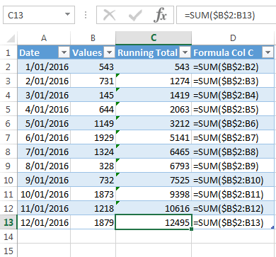
For example, the table below contains a running total formula in column C before I add a new row to the table (column D shows the actual formula in column C):
Now when I add a new record in row 14 the Table automatically grows, as it should, but the formulas that get auto-filled get a bit funky on rows 13 and 14:
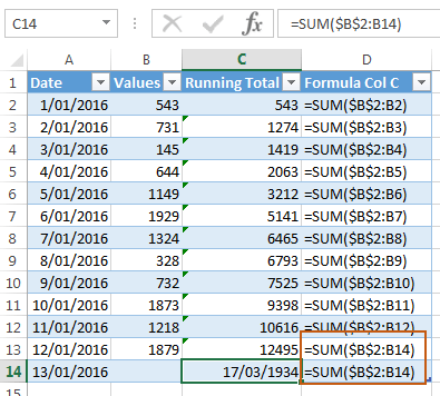
Not to mention the running total now returns a value formatted as a date. Huh?
You can see it before your very eyes in this animated image:
What’s also weird is if you remove row 14 the formula in row 13 corrects itself!
Excel Table Running Total Formula
Thankfully there’s a solution and it includes using the Excel Table’s own structured references.
Aside: Structured References are like dynamic named ranges that are automatically set up when you format your data in an Excel Table. They make working with Tables easy and efficient.
My Excel Table running total formula looks like this:
=SUM( INDEX([Values],1) : [@Values] )
We use INDEX to return the first cell in the Values column, and simply use the Structured Reference to the current row to return the second cell in the range we want to sum.
Note: [Values] refers to cells B2:B13 and [@Values] refers to the current row of column B. Learn more about Tables and Structured References here.
In English the formula reads:
INDEX the Values column and return the 1st cell : Return the cell reference to the current row of the Values column. And then SUM the values in that range.
If we were to step through the formula with the Evaluate Formula tool it looks like this:
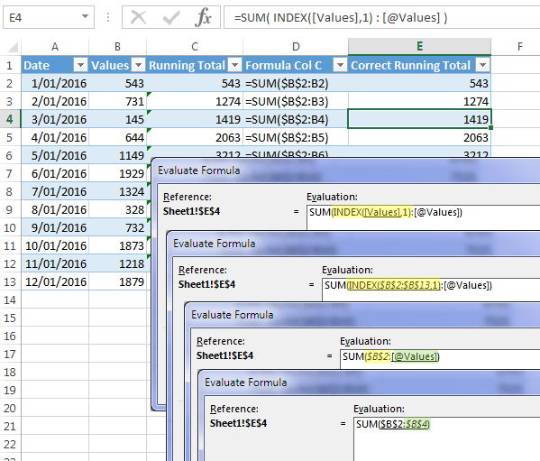
If you’re familiar with the INDEX function, for example you might have used it as an alternative to VLOOKUP, then you may be having an ah-ha moment right now as you realise that INDEX has actually returned a reference to a cell, and not a value like you might expect.
There's a lot more to INDEX than meets the eye. Check out these 5 secret features of the INDEX function:


Mynda, thank you for this tip. Very useful.
If I have a table where I am using this formula, is there a way to restart the formula after each month within the same table?
Karen
Hi Karen,
You’re best to use PivotTables if you want a running total that restarts with each month. You can use Show Values As in PivotTables for this.
Mynda
Mynda,
I like your “hide the zeros” number formatting. I’ve used formats like that since my Fortran work 40 years ago. A little thoughtful programming up front can make it far easier for the users later.
For Excel, may I suggest the following number format: 0;0;[color15]”•”
Why? Well…
1) This format hides the zeros
2) While making it clear the cell isn’t truly empty
3) And that we didn’t ACCIDENTALLY DELETE A FORMULA
4) By showing a light gray dot in place of a zero
Why a light gray dot? Well…
1) It’s inobtrusive
2) It’s not a common character and is unlikely to be confused with anything else.
3) It just shows the cell is occupied
I prefer the middle-sized dot [Alt-0149], but the small-sized dot [Alt-250] works, too.
BTW, in Fortran, hiding zeros wasn’t so easy, but the extra programming investment was worth not having to sift through acres of zeros in the output.
Nice! Thanks for sharing, David.
Mynda:
I really appreciate this tip, I have fought with trying to get this to work in tables for quite a while. I just usually ended up hard-coding the cell reference for the first cell, which sort of defeats the advantages of a table. Thanks!
Glad it was helpful, Glenn!
Why not use the same formula that the table totals field uses – in any non table cell =SUBTOTAL(109,Table1[col name]), works for all the examples I tried
Hi Terry, this tutorial is looking at running totals, not the totals at the bottom of the table.
Thanks Mynda,
I can now create my checkbook with:
SUM(INDEX([Credit],1):[@Credit]) – SUM(INDEX([Debit],1):[@Debit])
for the running balance.
Bob Marolt
Glad it was helpful, Bob!
Thank you so much for this! I’m creating a budget spreadsheet and I was about to settle for manually ignoring the errors in the total column but I thought – “there must be a way” and you helped me find it.
So pleased this tutorial was helpful!
very valuable formula Mynda! thanks!!!!
Thanks, Carlos!
Hi, thanks for outlining that solution. I’ve been a fan of Excel tables and the structure they bring for a long time now but the cumulative total has always been problematic.
I’ve used this approach for a while now but performance has become an issue as the table size grows since each cumulative cell has to sum ALL previous values to get the running total. Instead I came up with the following whereby the the current value gets added to the previous cumulative total while still using structured references as follows:
=SUM([@Values],INDEX(Table1[[#All],[Total2]],[@RowNumNo]))
where RowNum is another column defined as:
=ROW()-ROW(Table1[#Headers])
Note that the SUM function here simply adds two separate values, not a range. SUM must be used however so that an error is not generated on the first row when you try to add the header value to the current value (using a “+” operator does return an error).
This approach both results in a significant performance increase and makes the formula simpler to explain (possibly?) rather than introducing the concept of using INDEX to contextually return a cell reference rather than a value which might be quite new to many people.
This formula will NOT work with SUBTOTAL though so can’t be used to account for filtering (can’t immediately think how this might be handled and keep the performance but happy to hear any thoughts).
Good to know. Thanks for sharing, Hamish.
Hi Mynda – So can you please suggest how to amend this so the running sum picks up the first row when you apply a filter to the table? So the running sum gives a correct total.
Thanks
Dave
Hi Dave,
It’s not just the first row, all to rows should refer to the current row and the row above. What if the previous row is not exactly 1 row above, if the table is filtered?
See how the first value in a filtered list can be obtained here.
Thanks, you’ve saved my sanity! I was getting very frustrated trying to work out how to do a running total in a table and nearly gave up – then I found your tip.
🙂 glad I could help.
Thanks for the tip.
I was looking for something to create running totals for a grouping – I achieved this by replacing the 1 in your INDEX formula with a MATCH.
eg If there was a DEPT column in your table (so you want the running total to reset for a new DEPT), this should work:
=SUM( INDEX([Values],MATCH([@DEPT], [DEPT], 0)) : [@Values])
This presumes your data is sorted by DEPT.
Should work indeed, there can be a lot of scenarios.
Thank you for the tip.
How about identifying the row’s location using INDIRECT?
=SUM($B$2:(INDIRECT(ADDRESS(ROW(), COLUMN()-1))))
I’ve used this in other projects where I need to insert new rows, either in the middle or at the end of the table.
Hi Michelle,
Sure, that may work, but the INDIRECT function is volatile and therefore not recommended in large datasets, as it is likely to grind Excel to a halt.
Mynda
I use running totals in tables, but use SUM function without the absolute reference.
In Cell C2: =sum(B1:B2)
Since SUM() ignores text, it returns the first value and does the proper running total for all others.
Hi David,
If you copy your formula down to cell C3 you’ll get =SUM(B2:B3) and this won’t be a running total, it’ll only sum the next two cells.
Did I miss something?
Mynda
Header row is text value, so you can use this
=SUM(Table1[[#Headers],[Values]]:[@Values])
The same for COUNTIF and other functions…
Yep, Michael also offered that option. Cheers, eLCHa.
Nice trick. Is there something similar for Pivot Tables?
Hi Kevin,
PivotTables have a built in running total. Simply right-click the column you want displayed as a running total > Show Values As > “Running total in”.
If you also want the values not totalled you can add the column to the values area again so it’s displayed twice; once as a running total and once not.
Mynda
What’s the syntax for this formula if I want to place the it outside the table or if I have more than one table on the same sheet that has the same headings?
I was trying =SUM(INDEX(Table1[Values],1):[@Values]) but that produces an error.
Hi Stephen,
If your formula is outside the table then you can just use the regular running total formula:
=SUM($B$2:B2) and copy down.
But if you want to use structured references then the formula must be on the same rows as the table, as the @Values reference uses implicit intersection to resolve the actual cell. You can then use this formula:
Mynda
Thanks Mynda!
🙂
We may also use =SUM($B$2:[@Values])
Cheers 🙂
Sure can! 🙂
I am confounded. I can replicate the error using your spreadsheet, however I can copy your data to another spreadsheet, use your original formulas, and add all the rows I like and never replicate the error. I can even copy your data to another sheet or another spot on the same sheet and can not replicated the error.
Hi Jack,
Is your data formatted in an Excel Table? The problem only occurs in Tables.
Mynda
Yes it is. I have never noticed this phenomenon and so it interested me enough to play with it. I can copy your data to almost anywhere, retype the original formulas Sum($B$2:B2), and then Ctrl T and OK. Everything works perfectly. The only time it breaks is if I attempt to put the table in original position even after using Alt H, E, A to clear all. I am not knocking your work around but I am stumped on why I can’t recreate the issue anywhere but in the original position.
The formula only breaks when you try to insert a new row in the table. Did you test that step? If so, what version of Excel are you using?
Yes I tried inserting single rows and multiple rows, insert by dragging the bottom right cell and using the right click menu many times. The key is in your last question. I could not replicate your experience in Excel 2007 so I finally changed to another computer and Excel 2010 and there it was or at least something similar. If I inserted multiple rows, Excel would place the cell address of the last row entered into the first row inserted or if a single row it did almost the same as yours with the exception of the date thing.
Ah ha. Must be a version issue, starting with Excel 2010 and getting worse with 2013!
Nice trick, Mynda
Cheers, Alojz. Glad you liked it.
Thanks for this…I never knew this would happen. My running totals must have always been outside of a table! 🙂
I know it’s not as pure as your approach, but what about using nothing but structured references? In this case, since header rows don’t usually contain numbers, you can use that to your advantage:
=SUM(Table[#Headers],[Values]]:[@Values])
Oh…and for what it’s worth, although the formula problem persists, I don’t get the date formatting behavior in a table that I created in my version of Excel (15.25.1) on the Mac. But when I work with your spreadsheet, I do get the behavior. Not sure what the difference is…
Lots of things are different in the Mac version of Excel so I’m not surprised you get slightly different behaviour. I tested in Excel 2013.
Yep, that works too. Thanks for sharing, Michael.
Wo – mega helpful! Thanks for this tip!
You’re welcome, Nate 🙂
and if you want the sum of the last 2 values (yes, it’s happened!), you can use:
=SUM(INDEX([Values],MAX(ROW()-2,1)):[@Values])
assuming your table starts on row 1 – otherwise amend the -2
the MAX bit is to cope with the first table row which will otherwise give the whole column total
Interesting twist, Jim. Thanks for sharing.