Excel dynamic named ranges bring flexibility and efficiency to your spreadsheets.
Unlike static named ranges, dynamic named ranges automatically adjust in size as you add or remove data, ensuring that your formulas, PivotTables and charts always include the most recent information.
You can also use them to return different ranges based on selections in drop down lists.
If you frequently find yourself editing cell ranges that are referenced by formulas, PivotTables, charts, and other Excel features, then using dynamic named ranges will significantly streamline your workflow and save you a substantial amount of time.
Table of Contents
- Excel Dynamic Named Ranges Video
- Example File Download
- Excel Dynamic Named Ranges with INDEX
- Dynamic Named Ranges with INDEX Key Points
- Excel Dynamic Named Ranges with OFFSET
- Using Dynamic Named Ranges in Charts
- Troubleshooting Errors
- Relative Dynamic Named Ranges
- Alternatives to Dynamic Named Ranges
Watch the Video
Dynamic named ranges are a complex topic that are more easily understood if you can see them in action.
I recommend watching the video for the easiest way to get your head around them and then use the written notes below as a reference point.

Download Example Workbook
Enter your email address below to download the file.

Excel Dynamic Named Ranges with INDEX
Most people think of the OFFSET function for dynamic named ranges. Unfortunately, OFFSET is volatile, meaning it recalculates even if none of its arguments have changed, leading to more frequent updates and potential performance issues.
In general, it's a good practice to be mindful of the use of volatile functions, especially in large or complex Excel files, to ensure that they don't inadvertently slow down your work.
I prefer to use the INDEX function for dynamic named ranges.
INDEX has two syntax options, and for dynamic named ranges we use this version:
Syntax: =INDEX(array, row_num, column_num)
array – the range of cells you want to return a range from.
row_num – the row(s) you want to return.
column_num – the column(s) you want to return.
Applying it to this example data:
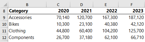
I like to write my dynamic named range formulas in a cell in the worksheet as it’s easy to construct them using the mouse to select the ranges and I can test they work as expected before defining them as a name.
Return a Range with Flexible Last Row and Column
This type of dynamic named range is useful as the source for PivotTables, and lookup formulas where you want to look up an entire table.
I can use INDEX with the COUNTA function to determine the current size of the table and return the range.
I’ve allowed for growth to row 16 and column L, as shown in the image below with the grey dashed line indicating the range that will be returned by the formula:
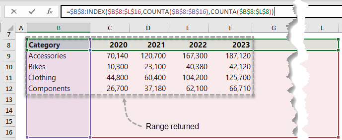
Each argument explained:
=$B$8
The first cell in the range I want returned. In this case it will always be the top left cell. Tip: if you don’t need the header row in the range, start at cell B9 and adjust the row_num COUNTA formula to also start in row 9.
:
Colon range operator.
INDEX(
Use INDEX to find the last row and column in the table using COUNTA for the row and column arguments.
array
=$B$8:$L$16
Select cells that represent the maximum size table will potentially grow to.
row_num
COUNTA($B$8:$B$16)
Counts the row labels in the first column to determine the current height of the table. The height of this range must match the height of the INDEX range and should not contain any empty cells.
column_num
COUNTA($B$8:$L$8))
Counts the column labels in the first row to determine the current width of the table. The width of this range must match the width of the INDEX range and should not contain any empty cells.
Note: when writing formulas for dynamic named ranges make sure the cell references are all absolute references.
Return a Range for a Specific Row
Sometimes you only need one row returned. It could be based on a selection in a data validation list or another cell, for use in a chart, table or a formula.
For example, below I can choose a different category from the data validation list and the values are returned and displayed in the chart.
Note: Excel 2019 and earlier users will not be able to display the values being returned by the formula in the grid (cells C38:F38) as you do not have dynamic array functionality. However, you can skip this step and simply define the formula as a name for use in charts etc.
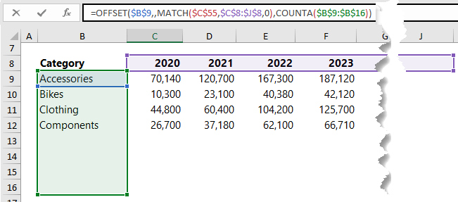
The formula for returning a range for a specific row uses INDEX and MATCH on both sides of the colon range operator:
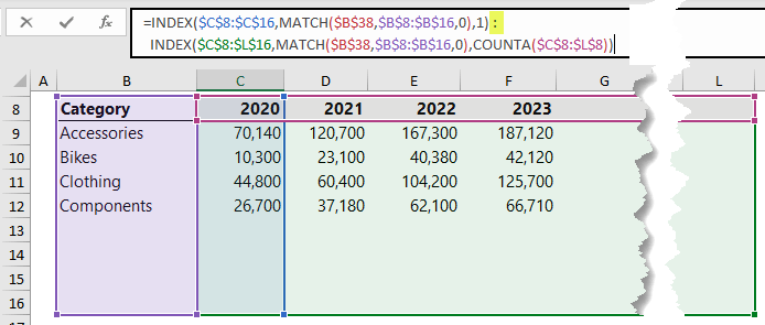
Each argument explained:
=INDEX(
Use INDEX to find the first cell in the range you want returned.
array
$C$8:$C$16
The first cell I want returned is in the first value column of the table (column C) and I’ve allowed the data to grow to row 16.
row_num
MATCH($B$38,$B$8:$B$16,0),
MATCH is used to find the row the category selected in cell B38 is on, in the range B8:B16.
column_num
1)
Technically this argument can be skipped as only one column is selected in INDEX’s array argument, but I’ve entered 1 for completeness.
:
Colon range operator
INDEX(
Use INDEX to find the last cell in the range.
array
$C$8:$L$16
The range containing the last cell, allowing for growth in rows and columns.
row_num
MATCH($B$38,$B$8:$B$16,0)
MATCH is used to find the row the category selected in cell B38 is on, in the range B8:B16.
column_num
COUNTA($C$8:$L$8))
Counts the column labels in the first row to determine the current width of the table. The width of this range must match the width of the INDEX range and should not contain any empty cells.
Return a Range for a Specific Column
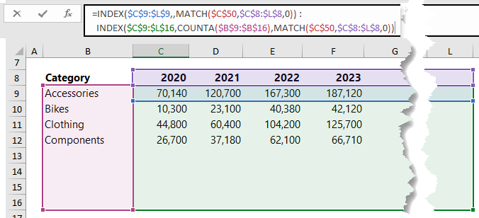
Similarly, we can use INDEX to return a specific column based on the selection made in the data validation list:
Note: Excel 2019 and earlier users will not be able to display the values being returned by the formula in the grid (cells C51:C54) as you do not have dynamic array functionality. However, you can skip this step and simply define the formula as a name.
The formula for returning a range for a specific column uses INDEX on both sides of the colon range operator:
Each argument explained:
=INDEX(
Use INDEX to find the first cell in the range.
array
$C$9:$L$9
The first cell I want returned could be in any column in the first row of the table and I’ve allowed the data to grow to column L.
row_num
This argument is skipped because there is only one row indexed, therefore a row_num is not required.
column_num
MATCH($C$50,$C$8:$L$8,0))
MATCH is used to find the column for the year selected in cell C50 in the range C8:L8.
:
Colon range operator
INDEX(
Use INDEX to find the last cell in the range.
array
$C$9:$L$16
The range containing the last cell, allowing for growth in rows and columns.
row_num
COUNTA($B$9:$B$16)
Counts the row labels in the first column to determine the current height of the table. The height of this range must match the height of the INDEX range and should not contain any empty cells.
column_num
MATCH($C$50,$C$8:$L$8,0))
MATCH is used to find the column that the year selected in cell C50 is in the range C8:L8.
Defining Names
The power of these formulas comes when you define them with a name. That name can then be referenced multiple times in formulas, PivotTables, charts and more.
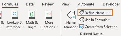
To define the formula as a name, make sure all the references are absolute. Then copy the formula > Formulas tab > Define name:
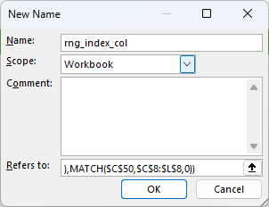
Name it and paste in the formula in the ‘Refers to’ field:
You can then reference the name anywhere you’d normally use a cell reference.
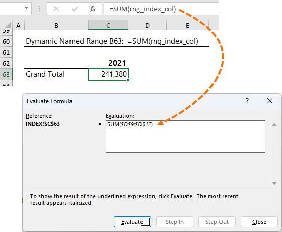
For example, in the image below I’ve summed the dynamic named range, and if I evaluate the formula, you can see that the defined name actually returns a reference to the range $C$10:$F$10
Dynamic Named Ranges with INDEX Key Points
Dynamic named ranges are incredibly flexible and with flexibility often comes complexity.
To summarize the key points:
- For dynamic ranges that you expect to grow, INDEX a range larger than the current data size and use COUNTA in the row_num and column_num arguments.
- For dynamic ranges linked to drop down lists or other cells where the user can specify what they want returned, use MATCH in the row_num and column_num arguments.
- If the start and end of the range need to be flexible, use INDEX on both sides of the colon range operator.
- Ensure all cell references are absolute before creating the defined name. There are exceptions to this which I cover in my Relative Named Range tutorial.
Excel Dynamic Named Ranges with OFFSET
The OFFSET function also returns a range that can be made dynamic with the use of the MATCH function and COUNTA.
However as mentioned above, it’s a volatile function and therefore should be used sparingly.
Let’s recreate the same dynamic ranges using OFFSET to see how it compares.
Syntax: =OFFSET(reference ,rows, cols, [height], [width])
reference – the starting cell/range of cells
rows – the number of rows to move +/- from the starting cell to arrive at the first row in the range.
cols - the number of columns to move +/- from the starting cell to arrive at the first column in the range.
height – the number or rows high you want the range.
width – the number of columns wide you want the range.
Return a Range with Flexible Last Row and Column
This type of dynamic named range is useful as the source for PivotTables, and lookup formulas where you want to look up an entire table.
I can use OFFSET with COUNTA to determine the current size of the table and return the range.
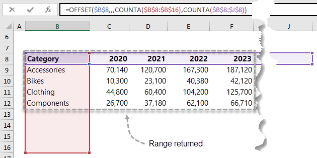
I’ve allowed for growth to row 16 and column J, as shown in the image below with the grey dashed line indicating the range that will be returned by the formula:
Each argument explained:
=OFFSET(
reference
$B$8
The first cell in the range will be the top left of the table.
rows
This argument is skipped because I don’t want to move down any rows from the reference cell before starting the range.
cols
This argument is skipped because I don’t want to move across any columns from the reference cell before starting the range.
height
COUNTA($B$8:$B$16)
Counts the row labels in the first column to determine the current height of the table. This column should not contain any empty cells.
width
COUNTA($B$8:$J$8))
Counts the column labels in the first row to determine the current width of the table. This row should not contain any empty cells.
Return a Range for a Specific Row
Returning a specific row that’s based on a selection in a data validation list or another cell, for use in a chart, table or a formula is also doable with OFFSET.
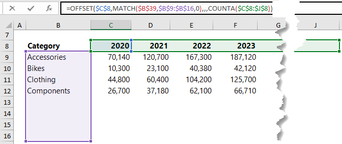
The OFFSET formula also uses MATCH to locate the row for the category selected in cell B39 and COUNTA to determine the current width of the table:
Each argument explained:
=OFFSET(
reference
$C$8
The first cell in the range will be the first Year column label. Notice the reference starts in the header row, because MATCH will return a value between 1 and 8, so at a minimum the starting cell will be 1 row below the reference cell.
rows
MATCH($B$39,$B$9:$B$16,0)
MATCH is used to find the row the category selected in cell B39 is on in the range B9:B16. The lookup range allows for growth in the table to row 16.
cols
This argument is skipped because I don’t want to move across any columns from the reference cell before starting the range.
height
This argument can be skipped because by default it will return 1 row.
width
COUNTA($C$8:$J$8))
Counts the column labels in the first row to determine the current width of the table. This row should not contain any empty cells.
Return a Range for a Specific Column
Similarly, we can use OFFSET to return a specific column based on the selection made in the data validation list:
Again, the OFFSET formula uses MATCH to find the relevant column and COUNTA to determine the height of the range.
Each argument explained:
=OFFSET(
reference
$B$9
The first cell in the range will be determined based on the year selected in the data validation list. Notice the reference starts in the row labels column because MATCH will return a value between 1 and 8, so at a minimum the starting cell will be 1 column to the right of the reference cell.
Rows
This argument is skipped because I don’t want to move down any rows from the reference cell before starting the range.
cols
MATCH($C$55,$C$8:$J$8,0)
MATCH is used to find the column the year selected in cell C55 is in, in the range C8:J8. The lookup range allows for growth in the table to column J.
height
COUNTA($B$9:$B$16))
Counts the row labels in the first column to determine the current height of the table. This column should not contain any empty cells.
width
This argument can be skipped because by default it will return 1 column.
Using Dynamic Named Ranges in Charts
One of the best uses for dynamic named ranges is as the source for charts, enabling them to automatically update as your data grows or selections are made.
However, there are a few tricks to getting them to work with charts.
- You need a separate name for the axis labels and each series’ values.
- You need to prefix the name with the sheet name followed by an exclamation mark:
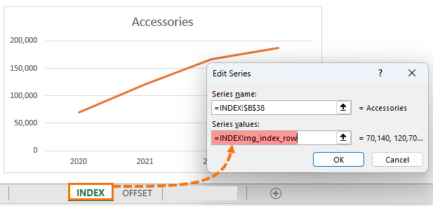
Note: after clicking ‘ok’ in the dialog box above, Excel will replace the sheet name with the file name.
Troubleshooting Errors
The 3 most common causes of errors with dynamic named ranges are:
- Erroneous data entered in the cells being counted for the height or width.
If you inadvertently enter some data below or to the right of your table inside the area being counted, you will end up with a range larger than it should be. - Blanks in the cells being counted for the height or width. The column you choose to count to determine the height of the range must not have any empty cells, otherwise the range will be smaller than it should be.
- Forgetting to absolute the cell references in the formula.
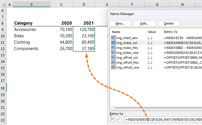
The easiest way to check the range being returned by a dynamic named range is to edit the range via the Name Manger (Formulas tab) and click in the Refers to field for the name you want to check.
Excel will put marching ants around the range being returned by the formula:
Relative Dynamic Named Ranges
So far, we’ve looked at dynamic named ranges that when referenced from anywhere in the workbook always return the same range. We achieve this by setting all references in the formulas as absolute.
However, we can also write relative named ranges that return a range relative to the cell in which you refer to it from and they’re particularly handy.
For more see my Relative Named Ranges tutorial.
Alternatives to Dynamic Named Ranges
Dynamic named ranges are a lot of work. It’s far easier to store your data in an Excel Table and use the built in Structured References that work like a dynamic named range by growing with your data.

I love your videos! So helpful and informative! Can you provide some instruction on how to deal with data that results from Excel’s new “array engine”. I like the convenience, but once a dynamic array is created, the data within it can’t be sorted or manipulated in any way, except to copy and paste it back as hard data. That defeats the whole purpose of formulas. Is there a “trick” to make data within an array result “manipulable”? Or does sorting, etc. HAVE TO BE done within the formula itself? Thanks, and please keep ’em coming!
Hi Peg,
Sorting can be done by wrapping the formula in the SORT function or SORTBY function, or you can reference the spilled array with the # operator and wrap that in SORT or SORTBY to return the array to another set of cells.
Mynda
I have used the OFFSET function before but it is particularly useful if you have dropdown validation lists that may require updating. You simply refer to the Named Range when setting up your validation. The dropdowns dynamically update without having to ammend your validation settings.
Hi, have you an example please!
Neither the offset nor index approach works with the SUMIFS function if the ranges contain blank cells in different rows. You can use either approach to perform a single operation on a single expanding range. SUMIFS is an extremely handy function. Thus far, I am using the primitive method of guesstimating liberally beyond my data. I have data, including many blank cells, in range A4:L1350. I am able to use SUMIFS, not with any of the OFFSET or INDEX formulas offered, but simply with the following:
=SUMIFS($G$4:$G$10000,$D$4:$D$10000,”*Item”,$C$4:$C$10000,”Person*”)
Thanks Mynda, I really like your step by steps !
I’m trying to set up a dynamic reference for a table with data re male and female. My goal is to build a chart with 1 serie with data re male and the other re female. Currently, each time I refresh the data, I sort the table by male/female then edit manually the graph series. Is there a way I could avoid that manual sort and let excel plot the “male” and female” series ?
Hi Sohpie,
I’d use a Pivot Table to summarise the data and automatically sort it. That way when you add new data it will automatically re-sort it. Make sure the PivotTable source data is formatted in an Excel Table so that when you add new data the PivotTable range automatically picks it up upon refresh.
If you get stuck please post your question and Excel sample file on our forum where we can help you further.
Mynda
Excellent article. A video could have been much better unless it is separately available
Great post, love the multiple options all explained thoroughly.
Just out of curiosity, on the offset example is there a reason for doing cell:offset cell rather than using the height functionality of the offset?
Hi Terence,
Thanks for your kind words.
There’s no particular reason for creating the range using cell:offset vs using the height parameter inside of OFFSET. I think I was just being consistent with the approach used to write the INDEX function dynamic named range, and so I wrote the OFFSET formula that way to make it easier to compare the two functions.
Mynda
Hi Mynda,
After studying your website and trying things out in the process of getting to terms with dynamic ranges, I seem to have created dynamic range names without using any functions at all, i.e. without Offset, Index or Indirect. This came as a surprise…
Starting with a copy of your raw data (columns A:E) I did the following:
1. Made a table of the raw data, including headings (Table1).
2. In column B: selected all Salesperson data excluding the heading and created a range name SalesPax with it.
3. In column E: selected all Order Amount data excluding the heading and created range name OrderAmt with it.
Both these are dynamic range names by virtue of being table data.
4. In Total Sales cell H2 used the formula =SUMIF(Salespax,G2,OrderAmt) which the system accepted and converted to =SUMIF(Table1[Salesperson],G2,Table1[Order Amount]).
5. Copied H2 to cells H3 through H8.
I’ve tested this by adding and deleting both Salespersons and Order Amounts to/from the original data table and all Total Sales in column H update correctly.
I welcome feedback on this approach. Thank you.
Regards,
George
Hi George,
Yep, that’s one of the features of Excel Tables. In fact you don’t even need to create named ranges. You can just refer to the table and columns using their Structured References. All explained here : Excel Tables.
Note: sometimes formatting your data in an Excel table isn’t ideal. For example, they aren’t suitable for data over 500k rows.
Mynda
There is (surprisingly!) another way to create this range using INDIRECT.
=INDIRECT(“B2:B”&COUNTA(B:B)-1)
While this bypasses the OFFSET function, it does require one to grasp the use of INDIRECT. In short, INDIRECT converts any text address as an actual address. Thus, it cannot be used by itself for it generates a #VALUE! error, the same one as the OFFSET function when used by itself.
Hi Bill,
That’s one of the great things about Excel. I would avoid using INDIRECT where ever possible though because it’s a volatile function and can cause performance issues in medium/large workbooks.
Mynda
Useful information,, cud u Plzzz post some samples, to Optimize data in Excel, for example PIPS data.
Hi Rajesh,
Sorry, I’m not familiar with PIPS data.
Mynda
Thank you, this was very helpful
I really like your explanation of the dynamic range name. Thank you for sharing.
Tim Hale
Cheers, Tim. Glad I could help.
I successfully applied the INDEX method in my files, but the named ranges disappear in the Name Box. What can be done to avoid this consequence of the INDEX method?
Hi Luc,
Dynamic named ranges never appear in the name box. It’s just how it is I’m afraid.
Mynda
I’m missing something here. I don’t see the advantage of using a dynamic named range rather than an Excel table. It seems to me the whole point of tables is that they are dynamic and “automatically” generate named ranges without the user having to identify ranges or use complex formula.
Hi Ed,
I too like using Excel Table’s dynamic structured references but Tables aren’t always an option so it’s good to know how to create a dynamic named range with formulas too.
For example, Tables can become very slow when they are a lot of formulas and are not always suitable for big data. They’re also not compatible with Excel 2003, although these days no one should be using Excel 2003 anymore 🙂
Kind regards,
Mynda
Mynda
I am trying to replicate what you have shown in excel_manual_chart_table, but there is no way I can do it. You seem to assume that one would intuitively know how to do all the things you show but the instructions are not detailed enough. For example, when I create the tow pivots tables, where do I put them? I notice that the chart for one table is sorted differently, but there was no instruction to sort anything. Sorry, I’m a beginner with pivot tables and charts, and I need step-by-step instructions, with nothing left to the imagination. Yet, this particular operation is very important to me. Hope you can help.
Arthur
Hi Arthur,
Great to see you’re having a go at replicating this technique.
If you’ve downloaded the file you’ll see where the PivotTables are in my file, however the location of them can be anywhere in the file. It makes no difference.
You don’t have to sort the PivotTable data, I just did because it’s useful to the chart reader. Sorting is easy, select a value (number) cell in the column you want to sort > right-click > sort > choose your sort order. You only need to sort the first PivotTable since the values from the second one are brought in using VLOOKUP and will therefore be sorted based on the first PivotTable.
Kind regards,
Mynda
Hi Mynda.,
These are great tools for dynamically naming ranges, and I love the way Tables are automatically dynamic.
What I’m trying to do though, is to use the offset or index function (based on a range in a separate sheet, and couple that with the table’s built in function, to make it automatically resize itself with the same amount of rows as my other range. That way, I imagine, the same way when you add data to the cell directly beneath a table, the table automatically resizes and copies down all the formulas of the other columns in the table, in this case, as I add a row to my “other” range on the other sheet, my Table will automatically add a line and copy down ALL formulas… even that for the first data point.
Sorry… I hope I was clear enough.
Thank you very much for all your help.
Hi David,
Great to hear you’ll be making use of dynamic ranges.
I’m struggling to picture the dependencies in your workbook. Are you able to send me a sample file with your question so I can better understand, and also give you a tailored answer? You can send it via the Help Desk.
Kind regards,
Mynda
Now when I think of all the old models where I used OFFSET in my dynamic named ranges I will dream about replacing it with INDEX based formulas as you outlined. Thank you for the tip!
🙂 great to hear, Joyce.
Hi Mynda ~
For anyone who routinely updates named ranges this is amazing! Of course, now that I’m trying to apply it, I’m stumbling. My first test file uses a named range in a vlookup. The current named range encompasses 2 columns (the first one is the lookup value [employee id], the second is the return value [employee name]) with data starting in cell B4 (header included). I attempted to use this formula for the named range but it errors out –=Employee!$B$4:INDEX(=Employee!$B$4:$C$4500,COUNT(=Employee!$b$4:$c$4500)). Either this won’t work across multiple columns or I’ve messed up the syntax somewhere. Would you mind pointing me back in the correct direction? Thanks!
Hi Leah,
It’s tricky to say for sure but, your formula contains = signs where they’re not required so let’s start by eliminating those so your formula looks like this:
Also, your INDEX formula is referencing B4:C4500 which is 2 columns, but you haven’t got a column_num argument in your INDEX formula. You either need to give it a column_num argument or make your range only 1 column wide.
Your COUNT function is also couting 2 columns: B4:C4500 you need to choose just the column you want to count, and if that column contains text as opposed to numbers then you need to use COUNTA instead of COUNT. COUNT only counts numbers.
If that doesn’t work then I’ll need you to send me the file via our Help Desk so I can see all of the contributing factors.
Kind regards,
Mynda
Thanks Mynda!
I modified the formula to this >> =Employee!$B$4:INDEX(Employee!$B$4:$C$4500,COUNT(Employee!$B$4:$B$4500),2) << and it worked! Absolutely fantastic. I can't wait to share it with my team.
That’s great, Leah. You should give yourself a pat on the back for mastering dynamic ranges using INDEX. Well done.
Mynda
Mynda: Another home run, mate! The Dynamic Range info is priceless (actually, I’m sure we could agree on a price!). 😉
Ken
Cheers, Ken. Just reaching for my calculator now 😉
I hv a question in setting range using table.
I hv a report which has 5 sections. Each section starts with a function, eg cell A10 = Admin. Each of the function has the same set chart of accounts.
Everymonth, I generate a new report, copy and paste the contents to a file which has formulae populating the data to a summary sheet in the same file.
The problem I hv is that when a new account is added to the chart of accounts, the range changes. I try to range each function using the table, unfortunately, when I copy and paste the new data, the table range seems hv removed.
Is there any other way to over come this problem?
thanks for your help.
rgds
Hi Rebekah,
Looks like you are pasting data over the entire table, including headers, this operation will delete the table. You should not do that, for example, if the first row contain headers, paste data under the headers row, starting from A2. This way, if you have extra rows, the table will autoexpand to include new rows, and even new columns (the new columns headers will be named automatically to Column1, Column2)
Of course, this assumes that the data structure is the same for the new data, and new columns are added to the right side of the table, not between initial data structure.
If the headers row structure is not the same, to preserve the table you can paste new headers to headers row, after you paste the data.
Catalin
Whoever from Microsoft Corp that invemted INDEX deserves a place in paradise. This function is gift from heaven.
🙂 Indeed, Maxime.
Minda, I never learne Excel but my level is very advanced. I am the Excel Guru at work, no joke. I can do most of the dashboards that I see online, I create my own, I helped all the departments in my organization using Excel, etc. I finally want to have a certification in advanced Excel with you guys. Can you send me the curriculum of your courses?
Another thing, what is the career of an Excel Guru? What should be his position in an organisation? What path should he follow? Please let me know. Thanks! 🙂
Hi Maxime,
It’s great to hear you are helping people get more out of Excel.
You can see our course syllabuses from the Pricing menu, then select the course you’re interested in. Each page with have a link to the syllabus.
Excel Guru’s come in all shapes and sizes and there is no definitive path. For example; you are already a Guru in your workplace. Helping out in Excel forums is a great way to increase your Excel knowledge. Typically the questions you find in forums are unique and challenging.
All the best with your journey to Excel heights.
Kind regards,
Mynda.
Thank you!
Hi Mynda, Really love your site. It has taught me so much already – especially the beautiful elegant way you have for explaining any topic. Such a contrast from the inbuilt Help with Excel.
Anyhow, I was wondering if you can help me out with a couple of queries on Dynamic Ranges and their application. Briefly, I have three worksheets (M,B,C) Each of them has an identical columnwise (15 columns) layout though the number of entries (rows) in each is different and is constantly growing. Hence I have made Dynamic Named Ranges (M,B,C) all with Workbook scope. Currently the number of rows of data (excluding Headers) for M is 25, for B is 60 and for C is 10.
Now I want to consolidate the three sheets such that all the data from M (25 rows across 15 columns) and B (60 rows across 15 columns) and C (10 rows across 15 columns) should be stacked one of top of the other i.e. excluding headers, row 1-25 should be M, row 26-86 should be B and row 87-97 should be C in a Master Sheet. Note-it should not sum the data but each individual row should be reflected in Master sheet such that Master sheet should have 97 rows and 15 columns of data. And thereafter as more and more rows of data are added to the 3 sheets, the Master sheet will incorporate all the entries (both old and new)
Is it even possible for Named Ranges to be displayed this way or can they only be displayed if some function is applied to them? Of course if it is not possible I would love to understand whether the issue is with the ranges being non-contiguous, being dynamic or their positioning on multiple worksheets or anything else. Intuitively I think it should be doable but I am unable to implement it.
VBA solution I have found is to create a temporary range which is a union of the three ranges but I would prefer to do it without VBA as multiple users will handle the document and are not as proficient/ comfortable.
Alternatively, a solution is to use multiple range/sheet inputs in Pivot tables – however, I am not able to get it to work as the page fields do not
reflect all the column headings the way it reflects when using a single input/sheet range. So solutions from this angle would also be welcome.
Thanks so much!
Keep up the AWESOMENESS!!
Hi Vinay,
Thanks for your kind words.
In regards to your question; I don’t know of a way to create a 3D dynamic named range. I’ve never seen it done and I can’t think of a way you could do it without VBA.
I would make all of your worksheets uniform and use PivotTables.
You haven’t said what you need this dynamic range for. I wonder if this tutorial on 3D SUMIF might be relevant.
Kind regards,
Mynda.
No Mynda, 3D Sumif isn’t relevant for this instance, although it seems like an interesting thing to learn.
I am not sure I explained myself correctly. What I am looking for is a way to consolidate multiple ranges together without summing them or any function. Just display the raw consolidated data one below another.
All worksheets are already uniform in layout – unfortunately I am not able to use the Pivot tables with multiple ranges as inputs as the page fields do not reflect all the column headings the way it reflects when using a single input/sheet range. Perhaps you have some suggestions/ tips for using inputs from multiple ranges/ worksheets?
Hi Vinay,
Yes, I know what you mean with consolidating PivotTables. Unfortnately the only other options are Copy and Paste all the data into one master worksheet, or find some VBA to do the copying and pasting for you.
Kind regards,
Mynda.
dear all. this code copy cell step by step. do you know any other way to write the code easier?
Hi Theron,
I really don’t think there can be any other, easier way of doing this code.
However, you may go to our HELP DESK and I’ll give you a file that could automate
some. Just specify what part of this topic explained do you want it to be
automated.
Cheers.
CarloE
a quick tip I picked up from another site for data validation
Lets say we are working with Range A1:A10 and A1 has the header to our list
Select A1:A10 and insert table (check the box “mt table has headers”)
(A1:A10 is now a table)
Select A2:A10 and name the range
Insert Data Validation in whatever cell you need it and input the range you named in previous step
thats it 🙂 you now have a dynamic range
If you add data to cell A11 it should appear in your drop down list
Hi Kevin,
Thanks for the tips.
Sincerely,
CarloE
Hi Mynda,
I have found the Dynamic Named Ranges using the INDEX function extremely useful, but have come across one small issue that you might be able to help me with. I have an excel based time-sheet for staff where they choose the site worked from a drop down list using Data Validation. As the number of sites is always changing I have named the site list using a dynamic named range using the INDEX function, but now find when you click on the drop down list you see the blank cells and have to scroll up each time to see the site list, is there a way around this?
Regards,
Keith
Hi Keith,
It’s good to hear that you have found it useful. I tried to simulate and walked through the file and I had a hard time trying to get
the same problem you have.
Anyway, It would be better for you to send your file through HELP DESK so we can have a better look at it.
Sincerely,
CarloE
Hi Keith,
First you need to create a list that doesn’t have blanks. Let’s say your list containing blanks is in cells A2:A9. In cell C2 enter this formula:
Enter with CTRL+SHIFT+ENTER as this is an array formula, and copy down as far as you need.
Then set up your dynamic named range referring to cells C2:??, let’s say C2:C1000 using this OFFSET formula:
Or using INDEX:
Kind regards,
Mynda.