No, no, no, no, no I’m not talking about the latest 3D animated movie.
I’m talking about how you can use SUMPRODUCT with SUMIF and INDIRECT to conditionally summarise data on multiple worksheets, for example when you’re creating a summary sheet in your workbook.
First the data:
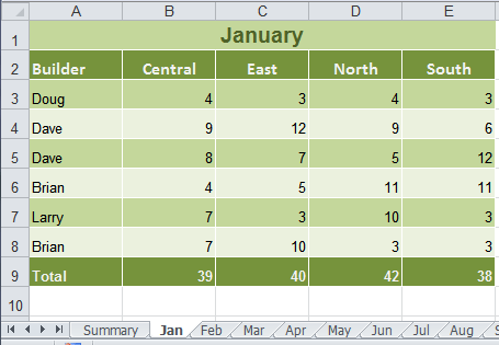
I’ve got 12 sheets just like the one below, one for every month – see the tabs at the bottom.
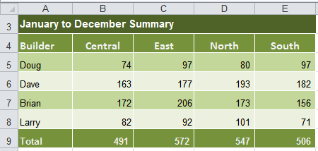
And I’ve got my summary sheet that totals up the data for each builder by region:
Here’s the problem (read ‘fun challenge’)
1. The data for each month contains multiple entries for some builders, so I can't simply sum it.
2. You can’t use the SUMIFS function across multiple sheets…well not on its own.
Solution 1: The slow option
If you’ve got oodles of time and a super computer you could add one SUMIF to another in one massive long formula like this:
=SUMIF(Jan!$A$3:$A$8,Summary!A5,Jan!B3:B8)+SUMIF(Feb!$A$3:$A$8, Summary!A5,Feb!B3:B8)+SUMIF……
Or.
Solution 2: The fast option
You can use a formula like this (from cell B5 of the summary sheet):
=SUMPRODUCT(SUMIF(INDIRECT("'"&tabs&"'!A3:A8"),$A5,INDIRECT("'"&tabs&"'!B3:B8")))
Enter your email address below to download the sample workbook.
Download the workbook used in this example. Note: The workbook download is a .xlsx file. If your browser changes the file extension to a .zip or .xml then you will need to replace it with .xlsx before saving the file.
How this formula works
I’m not going to go into massive detail as you can read up on SUMPRODUCT here, SUMIF here and INDIRECT here but I will to point out a couple of things.
If you know how to use SUMIF then you will recognise that cell A5 contains your criteria, in this case the Builder’s name.
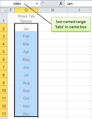
The other thing to note is the reference ‘tabs’. This is the named range given to the list of my sheet tab names located in cells G2:G13:
Note: you don’t need to give your list of sheet tabs a named range. You could simply reference the cells like this:
=SUMPRODUCT(SUMIF(INDIRECT("'"&$G$2:$G$13&"'!A3:A8"), $A5,INDIRECT("'"&$G$2:$G$13&"'!B3:B8")))
Back to why we need to create a list of sheet tabs…listing out the sheet tab names enables you to use the INDIRECT function to create the reference to each sheet on the fly, which results in a short elegant formula.
The Bad News
Because sometimes we have workbooks that contain a crazy number of sheets with complicated names you might be daunted by the idea of creating a list of the sheet names.
The Good News
Next week I’ll show you how to extract a list of your sheet tab names with some dead easy VBA. Seriously, it’s copy and paste kind of stuff.

I have information in different sheets and I need to have a summary , for samples , if I choose one day of the week , the resume show me the information that I have in the sheet 1 ,if I choose second day of the week the resume show me the information that I have in the sheet 2 .
How I can make the formula with 3D referent??
Hi Carlos,
The best tool for this is a PivotTable and Slicers, but you would have to consolidate your data onto a single sheet, rather than having it spread across multiple sheets. You can use Power Query to consolidate data across multiple sheets.
Mynda
I have a formula to summarize the reference across multiple worksheets as below:
SUM(‘Sheet1:Sheet5’!F352)
In case I would turn the reference “F352” to a dynamic range like “F”&TODAY()-44195, how could I put the assembled text “F”&TODAY()-44195 in the 3-D formula to replace F352. Thank you MYNDA I count on your brilliant guidance.
Hi Julian,
To create a range from text pieces, use the INDIRECT function, this returns a range:
=INDIRECT(“F” & TODAY()-44195)
My question is how to embed in the formula SUM(‘Sheet1:Sheet5’!F352)
to substitute” F352″, I tried to assign that INDIRECT function to a defined name “POS” then put it in the SUM function as follows:
SUM(‘Sheet1:Sheet5’!&POS)
but it didn’t work . I guess it must be incorrect join text and believe you can solve it. So, I come here!
SUM function needs a range, INDIRECT can return a range from text.
INDIRECT will not be able to create a 3D reference, so your sheets will have to follow a name convention:
=SUMPRODUCT(SUMIF(INDIRECT(“‘Sheet”& {1,2,3,4,5}& “‘!F” & TODAY()-44540),”<>0″))
This formula will sum Sheet1:Sheet5
Hi Catalin,
Many thanks to you. whether it be VBA or Function you alway come to my rescue with amazing solutions. I do appreciate it.
Br,
Julian
You’re welcome, glad to hear it works!
Cheers,
Catalin
SUMIF(‘1:10′!A:A,B4,’1:10’!B:B) kenapa nilainya Value
This was absolutely amazing and helped me so much, thank you! However, I am running into a problem with merged cells. The amount I need to sum is based on an account number (only one per sheet) but my criteria ranges are based off of an exception type and number of days past due (there could be multiple per account). If there are multiple exceptions for the account, the amount is only listed in the first row for that group of exceptions for the account and the formula does not pick up the amount if it is not on the same line. Is it possible to get the amount I need from a merged cell?
Hi Jared, glad you found this helpful. Merged cells are evil and should never be used for this very reason 🙂 I recommend you remove the merge formatting and enter the value in every cell. This is the correct way to structure your data. In fact, you really shouldn’t have your data spread across multiple sheets. The correct data format is tabular. I hope that points you in the right direction.
I agree! The problem is the Excel file is coming from Cognos and needs to be grouped by account and separated by lender on different sheets. They now want a summary for all lenders on a new sheet. If it wasn’t for the grouped/merged cell I’d be really happy. I did the same for counting items and it worked perfectly. I guess I’m going through 36 sheets and manually un-merging cells 🙂
Hi Jared,
You can also try Power Query if you have excel 2010+, to combine all sheets for reports.
After working on this problem for 5 hours and attempting so many longer versions, your recommendations help me get it done in 2 minutes. Wish your link was first to pop up on a google sheet for sumif multiple sheets.
So pleased we could help, Angelo! Just a shame you didn’t find us sooner. You can help our link appear higher up the search results by sharing this page 😉
I have a variation on this example that I can’t figure out. I have a year of data for each sales person in a by month format , so each sales person’s sales is on a separate worksheet with types of sales down column A and the months across the top – Jan 2019 Feb 2019 Mar 2019 etc. I need to consolidate the data on a summary sheet by sales (rows) and months (columns) across the top. My problem is that the months on each tab are in different columns. I could do this with sumif/index /match if the data were on a single sheet, but it doesn’t work using the 3D function using a table of worksheet names. I can send and example if not clear. Thanks for any insight.
Hi Rachel,
This is a classic case of your data not being in the right layout and it’s causing you all sorts of problems now that you want to summarise it. Ideally your data should be in a tabular layout. This will allow you to use PivotTables or SUMIFS to easily summarise the data.
You can use Power Query to unpivot the data and then consolidate it into a tabular layout.
If you get stuck, please post your question on our Excel forum where you can upload a sample Excel file and we can help you further.
Mynda
I’ve tried various approaches to 3D but can’t nail exactly what I want, which is to SUM the total HOURS spent at a SITE for a MONTH across 3 sheets (one for each contractor).
Most examples assume you have a different sheet for each month.
Main data source: Col.A = dates . Col.B = sites . Col.C = hours
Summary: Col.D = months
Columns E to K formula (each Site): total-hours-byMonth (E1=SiteName).
If I’m doing this on the individual contractor-sheet, the working formula looks like this:
=SUMIFS(C3:C10,A3:A10,”>=”&$D3,A3:A10,”<="&EOMONTH($D3,0),B3:B10,E$1)
Will it be possible to create a summary sheet?
=SUMPRODUCT(SUMIF(INDIRECT(…… etc.
Hi Anakowi,
I recommend you use Power Query to get the data from each of the sheets and consolidate it into one table so you can use SUMIFS the way it was intended, or even easier, summarise it with a PivotTable. If you really want to use a formula, then please post your question on our Excel Forum with your sample Excel file where we can help you further.
Mynda
Hi,
I hope someone can help. I’ve adapted the formula to the below but the result if #REF!
Can someone advise what I am doing wrong? I get confused with the use of ” and ‘ so any explanation would be helpful.
=SUMPRODUCT(SUMIF(INDIRECT(“‘”&tabs2&”‘!A5:A535”),$A6,INDIRECT(“‘”&tabs2&”‘!DY5:DY535”)))
Thanks in advance,
Lloyd
Hi Lloyd,
On the face of it the formula looks ok. We’d have to see the workbook to troubleshoot further. Please post your question and Excel file on our forum.
Mynda
Hi; Mynda;
I learned lot and enjoyed this article & other 2 articles. Thank you for writing so nicely.
Glad it was helpful, Mitul.
Hello,
I need help with the following requirement. I have multiple tabs and a summary sheet at the beginning. I am using the formula provided here to sum across the tabs on the summary sheet. However, new sheets are going to constantly be added to this workbook so the named range needs to automatically update as a new sheet is added. How can this be accomplished?
Hi Aubrey,
You can use this formula for the named range, it is dynamic:
=$G$2:INDEX($G$2:$G$500,COUNTA($G$2:$G$500))
I have been using the formula and have made a ‘named range’ for my worksheet names called ‘JuneNW’ (equivalent to your ‘tabs’). However, The formula is only using the value from the first worksheet (out of 17 sheets) instead of adding up the values associated with my ‘criteria’. Not sure if it matters that I am on google sheets instead of Microsoft excel. I have checked my formula countless times and it is identical to the one given above.
Hi Julianne,
We cannot help with Google sheets, the formula is designed for Excel, no idea if it works exactly the same on google sheets. You can try the formula in excel, you will have a comparison of the same file in excel and google sheets.
Catalin
Very useful formula. Thanks.
Hai guys.. I had experiencing difficulty in using formula sumproduct + sumif + indirect in calculating only “Actual” Total Sale on each sheet. Imagine that anybody can give a formula for the actual Total Sales data summarized into the Summay sheet. Examples of data on each sheet are as below.
Sheet1
Division Type Sales Retail
Division 11-Total Budget 792,510.00
Division 11-Total Actual 764,150.28
Division 12-Total Budget 1,358,200.00
Division 12-Total Actual 1,514,622.54
Division 13-Total Budget 1,322,000.00
Division 13-Total Actual 1,084,751.09
Division 14-Total Budget 49,000.00
Division 14-Total Actual 21,093.32
Sheet2
Division Type Sales Retail
Division 11-Total Budget 296,000.00
Division 11-Total Actual 265,594.15
Division 12-Total Budget 416,000.00
Division 12-Total Actual 305,710.21
Division 13-Total Budget 440,100.00
Division 13-Total Actual 527,700.01
Division 14-Total Budget 29,000.00
Division 14-Total Actual 11,126.42
Sheet3
Division Type Sales Retail
Division 11-Total Budget 473,000.00
Division 11-Total Actual 335,234.91
Division 12-Total Budget 394,000.00
Division 12-Total Actual 374,468.35
Division 13-Total Budget 829,154.00
Division 13-Total Actual 649,062.53
Division 14-Total Budget 56,000.00
Division 14-Total Actual 11,330.83
Sheet4 (Summary)
Division Total Sale(Actual) Total Budget
Division 11-Total
Division 12-Total
Division 13-Total
Division 14-Total
Hi Adrin,
Can you please upload a sample file on our forum? It will be easier for us to provide a functional formula and test it on your data structure.
Regards,
Catalin
Hai Catalin.. the sample file had been uploaded.. Topic name is “Need sum Sale (Actual) from multiple sheet”.
Hopefully getting feedback from you soon..
Thanks..
Looks like you already got a functional formula 🙂
Regards,
Catalin
Awesome! Thank you.
Hi! Could you help me with this modification?
In the function above can you use a criteria range instead of a single cell criteria?
like change the criteria in the function above from $A5 to A$5:A$9 or something
I have the same problem, but i want to sum based on multiple criteria. It seems to work on a single sheet but when i try to apply it in this formula it’s not working.
this is how i try:
=SUMPRODUCT(SUMIF(INDIRECT(“‘”&$G$2:$G$13&”‘!A3:A8”), $A5:$A9,INDIRECT(“‘”&$G$2:$G$13&”‘!B3:B8”))).
If i give a big criteria range it gives back “NA” error if i try a shorter range it gives back false numbers.
Thanks for the help!
Hi Daniel,
Can you upload a sample file so we can see what’s wrong? Use our forum to create a new topic and upload a file.
Catalin
This is great! now, how can I apply this concept using the INDEX formula so that my formula be more dynamic?
Hi Michaele,
Replace the named range ‘tabs’ with a dynamic named range.
Mynda
Thanks for the quick response. Maybe I didn’t frame my question right. I like the named range in the example above. And after using the formula more, and finding the ‘address’ function in comments/replys below to make it so the formula can be dragged over and the column update, I don’t need to use the INDEX formula. However, the example given below
(=SUMIF(INDIRECT(“‘”&$D$27&”‘!$B$1:$B$368″),INDIRECT($D$27&”!$A$375″), INDIRECT(“‘”&$D$27&”‘!”& ADDRESS(1,COLUMN(C1),2)&”:”&ADDRESS(368,COLUMN(C1),2)))
Doesn’t play well when a line gets inserted on the underlying tabs (it doesn’t update the range reference). Any thoughts?
Actually perhaps describing my use might be more helpful:
I am building a 10yr forecast model whereby there are underlying sheets (financial departments), which need to aggregate/roll up. I am familiar with INDEX combined with MATCH to pull back one value, but have not used it to pull back or aggregate multiple values from multiple sheets. Essentially that is what I am looking to do and I stumbled upon the above as a way to sum multiple tabs based on criteria.
In that case I would stop right there before it’s too late to fix the layout of your model. You should never spread source data over multiple sheets. Your source data should always be in a tabular format. This way you don’t have to wrangle Excel formulas to do things they weren’t designed for. Writing unnecessarily complicated formulas like this will only undermine the robustness of your model.
When your source data is in a tabular format you can easily use PivotTables to extract subsets of your data, or SUMIFS formulas to recreate those individual sheets, if that’s the final view you want.
Mynda
=SUMIF(INDIRECT(“‘”&$D$27&”‘!$B$1:$B$368″), INDIRECT($D$27&”!$A$375″), INDIRECT(“‘”&$D$27&”‘!C$1:C$368”))
In this formula if I want C$1:C$368 to change as per column(when dragging) , how to do that. Please help
Try this version:
=SUMIF(INDIRECT("'"&$D$27&"'!$B$1:$B$368"),INDIRECT($D$27&"!$A$375"), INDIRECT("'"&$D$27&"'!"&ADDRESS(1,COLUMN(C1),2)&":"& ADDRESS(368,COLUMN(C1),2)))Great tutorial.
I have made a formula to extract the tab names (to avoid VBA)
=RIGHT(CELL(“filename”;A1);LEN(CELL(“filename”;A1))-FIND(“]”;CELL(“filename”;A1)))
Then it is easy to refer to the tab names with a formula and changing the name of a tab will not cause the SUM IF formula to fail.
Nice tip, Soren. Thanks for sharing.
Mynda
I have few sheets within a workbook all having the same format.
Each sheet has Row 1 with B1..AF1 as date example from 1-May to 31-May
Column A2…A10 are various types of component names.
All sheets again uses the same date row and column name description.
We assume sheet 1 to sheet 3.
I want to create a summary page with Column description the same, but I just need to key into the cells selected as the following :
Sheet Name : just enter SHEET 3
Start Date: just enter 1-May
End Date: just enter 2-May
Once I key in the Sheet name with the date range selected, the Column will automatically show me all the total value of the quantity within the date range selected.
Can you help me on this?
Hi Fred,
Can you please upload a sample file to see your data structure? You can use our Help Desk (create a new ticket), it will be easier to provide a personalized answer, to match your structure.
Catalin
Hi Catalin,
Thk u for the prompt reply. I have already send my sample through the new ticket.
Regards
Fred
Great Formula!
Can I assume that the INDIRECT function is generating a multidimensional array that ultimately gets resolved by the SumProduct function? I tried using F9 to evaluate pieces of the formula but it doesn’t allow me to see the entire array.
Thanks
Yes, you got it right, INDIRECT will create a range from that text string.
If you select the entire argument of the INDIRECT function
"'"&tabs&"'!A3:A8"and press F9, excel will show the ranges created:{“‘Jan’!A3:A8″;”‘Feb’!A3:A8″;”‘Mar’!A3:A8″;”‘Apr’!A3:A8″;”‘May’!A3:A8”; “‘Jun’!A3:A8″;”‘Jul’!A3:A8″;”‘Aug’!A3:A8″;”‘Sep’!A3:A8”; “‘Oct’!A3:A8″;”‘Nov’!A3:A8″;”‘Dec’!A3:A8”}
If you select the entire function,
INDIRECT("'"&tabs&"'!A3:A8")and press F9, excel will give you the content of those ranges:{“Dave”;”Dave”;”Dave”;”Dave”;”Dave”;”Dave”; “Dave”;”Dave”;”Dave”;”Dave”;”Dave”;”Dave”}
If the range is too large, excel fails to display the data, there is a limit in the length of the text displayed.
Cheers,
Catalin
Hi,
This site is a great find and a gold mine of information. This process is very, very close to helping me solve what I want to do, but not quite.
I have a 12 tabs in a spreadsheet (one for every month) plus a summary/year-to-date (YTD) sheet where we track the sales of each of our 23 reps for three core product categories. Each month and rep also has a forecast for each core product category already built into each month tab.
What I want to do is a YTD “SUM IF” of the forecast fields in the Summary tab based on the month being processed. For example, if this is May 1, I would want to sum the forecasts for January through April only. Any suggestions are welcome.
Thank you!
John Galich.
Hi John,
Can you please upload a sample file with your data structure on our Help Desk? (create a new ticket). It will be easier to provide a personalized answer.
Cheers,
Catalin
Hi guys,
I am just starting with Excel, I know how to use formulas like sumif, indirect or sumproduct. But all of them by its own. I am trying to solve the example. As I am trying to really understand what I am doing, how can i use this kind of symbols, without just copying the formula that you give me?
”
“‘”
&
Thank you very much
Hi,
The single quotes (or apostrophy) are used in sheet names references, if the sheet name contains spaces , like this simple reference to a cell in another sheet:
=’Test Sheet’!B4 . If the sheet name does not contain spaces, the apostrophies are not needed: =Sheet1!A1
The double quotes are used in text strings, like: =”John Doe”
The & simbol is used for joining together multiple pieces of text, like:
=”John “&”Doe”
You will get the same result by using the CONCATENATE function: =CONCATENATE(“John “,”Doe”)
Hope this clarifies some things 🙂
Cheers,
Catalin
Thank you!
Just one thing. Like the example we are using:
…INDIRECT(“‘”&$G$2:$G$13&”‘!A3:A8″…
What I understand is:
“‘”= reference text which means nothing, no?, and
range G2:G13 and
“‘!A3:A8” another text reference with only one single quote
Hi,
A reference to a range from another worksheet looks like this:
=’Sheet 1′!A3:A8
Note that only the worksheet name is found between single quotes, before the exclamation mark.
In INDIRECT function, we recreate this reference structure by joining together multiple pieces of text strings:
=INDIRECT(“‘” & G2:G13 & “‘!” & “A3:A8”)
G2:G13 must hold the worksheet names list, as you can see we have to add a single quote before and after the worksheet names, folowed by the exclamation mark and range reference.
Cheers,
Catalin
Hi,
I have a worksheet and I was able to use this function perfectly. I just have an issue for some data that have codes within them. So for example in tab Jan instead of having Doug, I have WAVE_1 (Doug), and then for February it would be something like WAVE_2 (Doug), is there a way to use index match to find content within the cell instead of match the cell value?
Thank you,
Isabella
Hi Isabella,
Yes, probably, but I’d be inclined to separate the name out of the cells rather than try and coerce a formula into handling it.
You can use Text to Columns to extract the name in a few clicks.
Kind regards,
Mynda
Hi there,
Just wondering if this formula works if the ‘Dougs’ on Jan-Dec worksheets are in different cells.
So far, all Dougs are in cell A3.
What if:
Jan: Cell A3
Feb: Cell A16
Mar: Cell A9
Thank you!
Hi Winnie,
It will work if the ‘Dougs’ are in different cells in column A on each sheet.
Item 1 under the heading “Here’s the problem (read ‘fun challenge’)” says”
“The data for each month contains multiple entries for some builders, so I can’t simply sum it.” So therefore if you have your matching name in a different cell in column A it will work.
You just need to alter the range to include all the possible rows e.g. instead of A3:A8 make it to at least A3:A16, since your example says ‘Feb’ data is in cell A16. Likewise for the column B range. The formula below allows for up to row 100:
=SUMPRODUCT(SUMIF(INDIRECT("'"&tabs&"'!A3:A100"),$A5, INDIRECT("'"&tabs&"'!B3:B100")))Kind regards,
Mynda
Hi Mynda,
Thank you for this useful formula
Can you please tell me if there is a possibility to use this formula if central, east, north & South on Jan-Dec worksheets are in different cells.
Thank you
André
Hi André,
No, it requires the region to be in the same column.
Mynda
Hi Mynda,
This is a very interesting excel trick! But what is the purpose of having SUMPRODUCT in the formula? I know that the formula will not work without it, but can’t really figure out the reason behind it.
Can you please explain?
Thanks.
Hi Chee Teik,
SUMIF on its own can’t handle a 3D reference, but if you pass the resultant array to SUMPRODUCT it can sum up the values.
Kind regards,
Mynda.
Thanks Mynda, this really opens my eyes- SUMPRODUCT 3D.
I like your trick in creating the ‘tabs’ with INDIRECT. Nice! 🙂
Regarding your example, I would actually prefer Data Consolidation to setting formulas, given that the data in different worksheets are static.
What do you think?
Hi MF W,
Yes, you’re right. It’s different strokes for different folks.
However, I have my opinion that it’s easier to add one more item–builder in this case– and
in case of an additional sheet by just adding one more sheet name to the ‘tab’ range, and then just
copying the formulas without much ado to the new item(builder) to get the same results.
I think it’s harder — by a teenie-weenie only –for me to redo the formulas
to a new item(builder) using Data Consolidation in this case especially with an additional
sheet. But of course this is just my opinion and very negligible. It doesn’t really matter which you choose.
It’s just a matter on what you’re used to. It’s just like some people would prefer
keyboard shortcuts to a mouse.
Cheers,
CarloE
Excellent expaination of a very complex issue – thank you, that was very helpful.
Cheers, Mark 🙂
doesn’t work with NA() is cell… any alternative to sum cross sheets with NA() ?
Hi Diogo,
Get rid of the NA errors by wrapping the formulas in an IFERROR function.
Kind regards,
Mynda.
Hi,
How would you alter the formula so that instead of just typing in D2 and checking for one name in one cell across all worksheets (ie. Doug), it checked and matched two names in two adjacent cells (ie Doug Brown in D2:D3)
Hi Andrew,
First of all, I hope we are talking about the same file here: Excel_Blog_3d_countifs.
I don’t think it’s possible. SUMIF or even SUMIFS is designed only to evaluate a criteria range only once. For example,
If the ‘Builder’ column is evaluated as you suggested once for Doug and once for Brown, SUMIF could not perform an ‘Or’ mechanism rather if the same range
is to be evaluated twice it will not result into anything because it will require that both ‘Brown and Doug’ criteria be satisfied and not either.
I hope it’s clear because I am not good at explaining 🙂
Cheers,
CarloE
I need to track multiple tabs for both a date range and a name range. Working in one workbook, I have a tracking tab to summarize and the tab names are years (say 2002- 2013). I wanted to use the INDIRECT formula but am running into a road block. If I have a dynamic name range indicating a list of tab names. Should I be putting a name range on each tab as well? I have had to use the actual tab name to track but only am getting half way there. I can track date ranges from each tab but not name and date ranges together. (the list of dates and names also exist on the tracking tab for an easier formula.) Heres what I have so far.
=COUNTIFS(‘2002′!$M$3:$M$12081,”>=”&E$17,’2002’!$M$3:$M$12081,”<="&E$18)
Can you help?
Hi stonecottage,
Please send this file here: HELP DESK.
Please explain your problem further.
Cheers,
CarloE
Hi there Mynda,
I’m having a problem with a workbook that i am working on and here is my scenario.
I have a range of tables across multiple sheets that all reflect safety stats. Each sheet has the same layout and structure and applies to different site locations. Each sheet is accompanied by a corresponding ‘graphical’ sheet which illustrates the stats in a graph.
What i am idealy attempting to do is to create a summary page using the same structure and tables as the site pages, yet summing pertinent values from the various sites.
EG hours worked is B Column and the first value occurs in B3.
I’m wanting to SUM the vaules from all the relevant site pages into the summary page, whilst excluding the graph pages.
Additionally i’m wanting the formula to have drag down functionality.
I was thinking that sumproduct or the sumifs would be a good solution – yet a lot of the syntax here is going over my head.
Any help with a solution would be much appreciated
Kind regards
Tobias Ford
Hi Tobias,
Please send this through HELP DESK.
It would be easier if we can see this on file.
Otherwise we can only advise to go and read our posts
–and you guessed it right–:
SUMPRODUCT
SUMIFS
Cheers,
CarloE
PERFECT!!!! THANK YOU!!! YOU SAVED ME!
Hi Mihaela,
On behalf of Mynda,
You’re welcome!!!
Carlo
Looks very good
Cheers, Berry 🙂
I have studied the functions used in this and I don’t understand why you use sumproduct AND sumif, why can’t you use sumproduct and indirect on their own?
Hi Stephanie,
Sumproduct can be use on its own with INDIRECT. However, for some weird reasons, It doesn’t work like the SUMPRODUCT,SUMIF,INDIRECT combined.
In short, Sumproduct can only use a 1-celled dynamic range. For example, In our article, We cannot use the ‘tabs’ range which has 12 months(data in it).
If you have downloaded the file already,
Try this variation in E5.
=SUMPRODUCT(INDIRECT(“‘”&tabs&”‘!E3:E8”)*(INDIRECT(“‘”&tabs&”‘!A3:A8”)=$A5))
you’ll get an ERROR. lol. but that’s not it.
Goto Formulas Ribbon, Name Manager, CLick ‘tabs’ and edit its range to just $G$2.
you’ll see that your error changes to 3 which is the value of Doug for the Jan sheet.
To be honest, I don’t know why it’s like this. I guess, SUMPRODUCT is way too complicated
a function that its creator just wanted to limit its range. Its complication is that you
can use +(OR) and *(AND) operators in a very diverse kind of way. Incidentally, SUMIFS will work
too despite its multiple criteria ranges/criteria feature. I guess -again- it’s more
predictable unlike SUMPRODUCT. Who knows someday they’ll improve this limitation.
Sincerely,
CarloE
SUMIF FORMULA is =SUMPRODUCT(SUMIF(INDIRECT(“‘”&A2&”‘!O:O”), B2, INDIRECT(“‘”&A2&”‘!AE:AE”)))
Where
1 A2=SHEET NAME
2 O:O= CRITERIA RANGE
3 B2=CRITERIA
4 AE=SUM RANGE
Hi Rashid,
Do you have a question or are you just making a statement?
Cheers,
Mynda.
Hello Mynda,
I’ve followed your advice, created a group named ‘tabs’ and listed all of the tab names in it.
I’m using several summary sheets in which I am adding wins and losses in the following groups: Overall, Conference, and Division. Your formula works perfectly for Overall and Conference wins and losses (which are in separate columns, i.e. Overall wins, Overall losses, Conference wins, Conference losses).
For Division wins and losses, my reference range is different, where instead of referencing a range of 12 cells, I’m using a range of six cells (also on the same spreadsheets). For some reason, the totals are not adding up for this group and I can’t figure out what’s different.
For the North Division wins, my formula is: =SUMPRODUCT(SUMIF(INDIRECT(“‘”&tabs&”‘!V2:V7”),$A4,INDIRECT(“‘”&tabs&”‘!P3:P14”)))
While for the South Division wins, the formula is: =SUMPRODUCT(SUMIF(INDIRECT(“‘”&tabs&”‘!V9:V14”),$A4,INDIRECT(“‘”&tabs&”‘!P3:P14”)))
V2:V7 & V9:V14 reference a spot on the ‘tabs’ worksheet where I have division standings. The ranges are correct, but the totals aren’t — that is if the team has a total >0. It is totalling ‘zero’ just fine.
Can you help?
Hi Rob,
I have tried some experiment on my own but It would be better if you send me the file through Help Desk so I can see the flow or logic of your formulas and the data it is based upon.
Sincerely,
CarloE
Hi Carlo,
Thank you! I’ve submitted a ticket and attached my file.
Hi Rob,
I was quite lost there for awhile. 😉
Anyway, you said that your range V2:V9 is correct, but I beg to disagree because you’re using a SUMIF.
SUMIF works only if the rows of the sum range and the range criteria are of the same dimension.
in your case V2:V7 being the criteria could not locate P3:P14 except I guess between P3:P7 which would
qualify as of the same dimension–that is why I think It picked up several figures.
=SUMPRODUCT(SUMIF(INDIRECT(“‘”&tabs&”‘!H3:H14”),$A4, INDIRECT(“‘”&tabs&”‘!P3:P14”)))
So that solves why your SUMIF isn’t working.
As to the expected, next problem…
I suggest — it’s just a suggestion– that you have a master list as to who’s in ACC North and who’s in ACC South. In that way we can easily put teams in the right division using an IF Function directly in your ACC Sheet… i.e. IF Virginia is North then our SUMPRODUCT function else 0. something like it.
I am saying this because I have tried to use the SUMPRODUCT using a combo of INDIRECT, ISNA,ISERROR,VLOOKUP and it just provided an inconsistent result… and I don’t know why.
Sincerely,
CarloE
Hi Carlo,
Thank you for looking into this for me. I didn’t consider the restrictions in range and your explanation makes perfect sense.
If I can figure out how to look up a value in ranges x and y, then pull the information from range z, do this for a range of tabs adn sum the figures, then take that corresponding value and put it in either section a or b (depending on where finding the value(s) in x or y) of the summary sheet, I’ll be all set.
Hi Rob,
Do you still need help on that? I’ve been doing something like that last week and I got inconsistent results. I think I can do it on a sheet per sheet basis but not on a range of tabs using INDIRECT.
I will still try though. Do you like a customized VBA function?
I will send it to you through helpdesk.
Sincerely,
CarloE
Your formula =SUMPRODUCT(SUMIF(INDIRECT(“‘”&tabs&”‘!E18:E190”), $H8,INDIRECT(“‘”&tabs&”‘!g18:g190”)))
Works brilliantly for me but i need to amend slightly so that the formula counts the number of items in G18:G190 rather than sums them up. Replacing SUMIF with COUNTIF unfortunately doesnt work.
Also I need to amend the formula after that to count the number of items that are in I18:I190 (instead of G18:G190) that have the word “Bound” in it.
Any thoughts?
Hi Nick C,
I am sure I have answered a similar question before and I thought it was you but
I couldn’t find the thread.lol
Anyways, Nick try to position your cursor in your current formula and “CTRL+SHIFT+ENTER”
that will make an array formula of countif.
Read : Array Formulas
Cheers.
CarloE
I have figured out my count issue above – but i do need help on a sumif (or sumifs) query
=SUMPRODUCT(SUMIF(INDIRECT(“‘”&tabs&”‘!E18:E190”),$H10,INDIRECT(“‘”&tabs&”‘!g18:g190”)))
the above formula has a condition that H10 needs to be in the E18:E190 range.
Why does my formula BELOW not work to have an additional condition that H11 needs to exist in range B18:B190?
=SUMPRODUCT(SUMIFS(INDIRECT(“‘”&tabs&”‘!E18:E190”),$H10, INDIRECT(“‘”&tabs&”‘!B18:B190”),$H11, INDIRECT(“‘”&tabs&”‘!g18:g190”)))
Hi Nick,
Your syntax is wrong.
SUMIFS and SUMIF are two different things; Although, It shows similar results.
SUMIFS Syntax: SUMIFS(SUM Range, CriteriaRange1, Criteria1, CriteriaRange2, Criteria2…and so on)
In your case you’re trying to treat SUMIFS like it’s a SUMIF.
Cheers.
CarloE
Dear Mynda
Thank you very much for the brilliant work. I have two follow up questions. First, how do I write this formula if I want to locate this named range (“tabs”) on a different page from the formula? Ex. Formula is on worksheet named “summary” and the tabs named range is on worksheet named “tabs”. Second, if it is possible to name this formula, something like =Formula(J23), would it reduce the size of my file (now 300Mb)? Because I have to make this calculating the formula over 10000+ rows. I am having a very difficult time trying to figure out the syntax involved in the indirect function. What are the best tools to use to tutor myself? TIA
Hi PT,
You can put the tabs list on any sheet, just make sure when you give it the name that you set the ‘Scope:’ to Workbook.
You can read a tutorial on INDIRECT here.
In terms of giving the formula a name to reduce the workbook size, I don’t think it will work. Excel still has to perform the calculation 10000 times. SUMPRODUCT is known to be labor intensive for Excel when crunching through large workbooks.
I’m not sure of your exact formula but if your workbook is slow make sure your formula doesn’t reference any whole columns. Only reference the cells you need so that Excel isn’t doing any redundant calculations.
I hope that helps.
Kind regards,
Mynda.
Dear Mynda:
Hi its me again, PT. If have been very productive with versions of your formula above since my last question, because of your help. I am still finding Indirect intuitively challenging. My question. As a background, I originally had 10 worksheets and a single summary sheet in 1 file. Then I split off the 10 worksheets and put them into their individual workbooks (the single file would no longer open and my OS would freeze). So now I have 10 workbooks and a Summary workbook. Now I would like to take the formula from above:
=SUMPRODUCT(SUMIF(INDIRECT(“‘”&tabs&”‘!J”&ROW(J23)),”>0″, INDIRECT(“‘”&tabs&”‘!J”&ROW(J23))))
And create a Named Range for column “J” in each of the 10 workbooks. By doing this I figure I can insert new columns between “A” and “J” without having to rename every column that appears after “J” in my Summary workbook (i.e. columns K, L, … DA). Each column including column J is the same for each of the 10 workbooks. I have tried several formulas but I receive #REF! and #NAME! responses. For example I tried renaming every column J in the 10 workbooks, from row 2 to row 15,000, the name “Ticks” and then summing all the column J’s in the Summary file with the following formula:
=SUMPRODUCT(SUMIF(INDIRECT(“‘”&tabs&”‘!”& Ticks&ROW(J23)),”>0″, INDIRECT(“‘”&tabs&”‘!&Ticks&”&ROW(J23))))
If you could assist me I would very much appreciate it.
TIA
PT
Clarification: the bottom formula is
=SUMPRODUCT(SUMIF(INDIRECT(“‘”&tabs&”‘!”&[Stock1.xls]Ticks&”!”&ROW(J23)),”>0″, INDIRECT(“‘”&tabs&”‘!&[Stock1.xls]Ticks&”!”&ROW(J23))))
TIA
Hi PT,
It’s easier if you can send me the file. Can you please log a ticket on the help desk and attach the file.
Cheers,
Mynda.
Hi Mynda,
I have tried your formula but it is not working for my challenge, so I am asking you for help.
I have 10 worksheets in an excel 2003 file, each representing a stock (i.e. 10 stocks), and each row represents one trading day, and each column represents different data or formulas derived from the data during each day. In column “J” of each day of each sheet, I get either positive or negative number. For example cell J23 on each sheet might contain -4, 2, 10, -3, -6, -5, -3, 6, 1, 1 (or whatever the case may be).
Then I have a summary sheet (worksheet 31) in which I would like to add up all the numbers that are negative, and all the numbers that are positive. In the example my two formulas should give the results -21 and 20. For the negative calculation I tried
=SUMPRODUCT(SUMIF(INDIRECT(“‘”&Sheet1:Sheet10&”‘!J23:J23”),J23<0, INDIRECT("'"&Sheet1:Sheet10&"'!J23:J23")))
That's it. How do I do it? Can you help?
Just a clarification, worksheets 11 through 30 are all unrelated sheets. While my summary sheet is worksheet 31, it could be any sheet.
Hi PT,
You need to list the sheet tabs somewhere in your workbook and give them a named range, e.g. ‘tabs’. You then use that named range in your formula instead of ‘Sheet1:Sheet10’. Like this:
=SUMPRODUCT(SUMIF(INDIRECT("'"&tabs&"'!J23"),">0",INDIRECT("'"&tabs&"'!J23")))You can also download the Excel workbook used in the example above and have a look at what I did.
Kind regards,
Mynda.
Thank you Mynda. The formula works! However, I cannot copy the formula to the next row because the J23 remains J23 and does not change to J24, or J25, and so on. What should I do? TIA
Hi PT,
Here’s the formula for adding up cell J23:
=SUMPRODUCT(SUMIF(INDIRECT("'"&tabs&"'!J"&ROW(J23)),">0",INDIRECT("'"&tabs&"'!J"&ROW(J23))))You can then copy this down the column.
Kind regards,
Mynda.
This post has been very helpful. Thank You. For the formula below, where you add the Row function to make the formula dynamic so that it can be copied. How do you enable it to be copied when it needs to cover a range (as opposed to just one cell as it is below)?
Thanks again.
Chris
Hi Chris,
Glad you found it useful 🙂
You can simply reference a range in the ROW function like this: ROW(A1:A10)
If you want the ROW function to always start at A1 then modify it to: ROW($A$1:A10)
Likewise if you want it to always reference A1:A10 then modify it to: ROW($A$1:$A$10)
Kind regards,
Mynda.
I AM TRYING SUMPRODUCT PROPER FORMULA BUT ANS IS REF# DON’T KNOW WHY IS THERE ANY HELP FOR ME
Hi Kibria,
You usually get a #REF! error when one of the formula parameters is pointing to an invalid range.
Kind regards,
Mynda.
Or a blank cell in the list of cell names
Bravo!
🙂 Cheers, Luis.
The indirect part should be INDIRECT(“‘”&A1&”‘”&”!E:E”) for the apostrophe. It works