The Excel INDIRECT Function has many applications and perhaps its simplest is to fix a range of cells you want to reference.
For example a standard SUM function looks like this:
=SUM(B16:B24)
If you insert a row within this range the formula dynamically updates and becomes:
=SUM(B16:B25)
It will dynamically update even if you absolute the reference like this:
=SUM($B$16:$B$24)
To stop the reference dynamically updating when you insert rows or columns use the INDIRECT function like this:
=SUM(INDIRECT("B16:B24"))
In most cases you’d want your formulas to dynamically update when you insert new rows or columns but there are some instances when this is a nuisance and that’s when INDIRECT is your ally.
How Does The INDIRECT Function Work?
Excel’s INDIRECT function returns a reference specified by a text string.
The text string can be obtained by:
- referencing another cell, or
- you can enter it in double quotes, or
- you can generate it by nesting other functions
You can also use the ampersand (&) symbol to concatenate text and build your text string that way. More on using the ampersand in a moment.
Notice how the range specified in the INDIRECT function below is surrounded by double quotes, thus making it a text string.
=SUM(INDIRECT("B16:B24"))
INDIRECT Function Syntax
The syntax is:
=INDIRECT(ref_text,[a1])
ref_text – is the text string (like in the example above "$B$16:$B$24") or the cell you’re referring to containing the text string.
a1 – this is asking you if your reference uses the A1 reference style or R1C1 style. To use the A1 style* simply omit this argument, but if you want to use R1C1 enter ‘FALSE’.
*A1 reference style is what you’re probably familiar with and it is where the columns have letters and the rows have numbers. The R1C1 style uses the R to specify a row and then the number of that row, and the C to specify a column and then the number of that column.
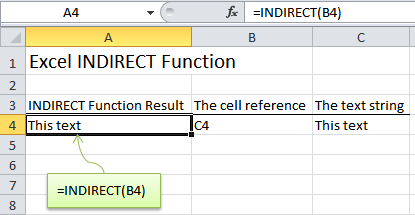
In the example below the INDIRECT function in cell A4 is evaluating the contents in cell C4. I could have also typed this formula like this:
=INDIRECT("C4") and my result would again be ‘This text’.
Ok, that’s enough theory.
Other Uses for INDIRECT
1. Generate a Reference on the Fly
By nesting it with other functions we can generate references like this one:
=SUM(INDIRECT("B27:B"&ROW(B35)))
In this example we’ve used the ROW function which returns the row number of the selected cell, in this example it’s 35. Our formula above evaluates to:
=SUM(B27:B35)
Well why didn’t I just type in =SUM(B27:B35) I hear you say. And fair enough too.
The point of this example was to give you a taste of how you can nest other functions in the INDIRECT function to derive cell references. I recommend you try nesting other referencing functions like COLUMN, ADDRESS, and CELL.
Referencing Other Worksheets and Workbooks
You can reference other worksheets and workbooks with the INDIRECT function too.
References to other workbooks must be formatted like this:
=INDIRECT(" '[your_workbook_name.xlsx]your_sheet_name'!$A$3")
References to other worksheets must be formatted like this:
=INDIRECT(" 'your_sheet_name'!H34")
Note 1: spaces between double quotes and apostrophe (“ '[your) are so you can clearly see all of the components. You don’t actually put a space in your formula.
Note 2: you can reference other worksheets and workbooks but if you reference another workbook it must be open otherwise you will get a #REF! error.
2. Use INDIRECT with a Named Range
This is probably the second most useful application for the INDIRECT function.
Let’s say you’ve got 4 named ranges of data; North, South, East, West.
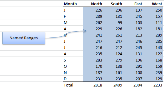
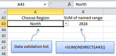
You’ve got a drop down list (data validation list or combo box) that allows you to choose from the 4 different regions (with names that are exactly the same as the named ranges you’ve set up for your regions).
When you make your choice the report automatically updates with the relevant figures without the need for any IF Functions or other jiggery pokery.
You can use the INDIRECT function in any formula that requires a reference to a cell or range of cells.
Download the Workbook
Enter your email address below to download the sample workbook.
Download the workbook and look at the examples in more detail.

In this formula =INDIRECT(“Abst!Z”&AD8+3) I want to add MG/DL. How can I do that? I tried =INDIRECT(“Abst!Z”&AD8+3)+”MG/DL” & few other combinations.
Hi,
You can build references from text only inside INDIRECT argument, can you clarify what + “MG/DL” should do?
My guess is that “MG/DL” means “milligrams/deciliter” and if that’s right, you can add it to the output in several ways. One is better than the other.
A first way to consider is that you could, of course, concatenate (or concat, or even textjoin) it to the basic calculation by adding:
&” MG/DL”
to the end (for example, after the “3)” at the end), much as you tried starting with the “+”… it’s just that “+” is inappropriately used there as it only does addition and not concatenation.
This adds to the formula complexity, but if the measure can change, adding it to the formula can help vary the measure for each value (there’s be some work to do, but it could be done relatively easily). However, it would be odd, probably, for such a thing to be needed in a table and you don’t really indicate a need for it. So maybe not much of a benefit.
However, it the need could arise, especially if the output is used in text in some way, outside the presumed table, it could be handy.
A second way would be to simply format the column with the measure in the formatting string. For instance:
#,##0.00″ MG/DL”
which would give results with the measure appended to them. So no need to add anything to the formulas, and so no extra work being done making the spreadsheet or by Excel whilst working. NOT as helpful if the result is going into text, like in a letter or report, rather than a table. But you can wrap the result in the TEXT() function, using a string like the above, for that.
The huge advantage is that the result in the table stays a NUMBER rather than becoming text by adding text to it. So the values can be used going forward in your process. If not needed, well, not as huge an advantage.
A third way would be “out of world” as one says. It would not use Excel’s formulas or even formatting to indicate the “MG/DL”: simply add the measure into the column title. Don’t mess with the calculations. Just add it to the title so the title reads something like:
Dorpurs
(MG/DL)
You know, if “Dorpurs” are being reported. Otherwise, use the right label!
Everything stays a number, no complexity is added to the formula, there’s less to maintain over time, and if the results are used forward into a letter or report, say, the formula there can have the complexity, or it could be part of the text in the template. If “mail merging” it into a Word document, Word has a FIELD that can do it.
Like all things in life, the exact choice is up to the details of the exact situation. But if aware of the options beforehand, one might choose to build something that will lead to using the easiest option available. If not aware of (some — there’s likely ten other ways to do this, or more!) options, one might have a hard time even conceiving to use an option, much less building toward it.
Hi there,
I have a summary sheet where I intend to populate data from 25 sheets i.e. AA, AB, AC, AD and so on. My Cell 30 of Sheet AA = “Canada (150)”. I used following the formula to extract “Canada” and “150” in separate fields.
Canada = LEFT(C30,FIND(” (“,C30&” (“)))
150 = (MID(C30,SEARCH(“(“,C30)+1,SEARCH(“)”,C30)-SEARCH(“(“,C30)-1))
I am wondering if I could use INDIRECT Function to extract data. Kindly advise.
Hi Taha,
INDIRECT is meant to allow you to create cell references from text strings, not for extracting data, with its specific advantages and disadvantages. To extract data from a large number of sheets, Power Query is your friend, if the structure is the same in all sheets. If you don’t have the possibility to use it, you can use as you said the INDIRECT function to build a 3D reference, have a look at this tutorial
Catalin
thanks fully
Mynda – This function is considerably more practical for my current need than a series of embedded IF statements. I would never have even thought to look for a function like this without your tutorials. Thanks so much!
kayakbob
Thanks, Kayakbob 🙂 Glad to have helped.
very good introductory lesson on indirect function. one can work on it. extremely usefu. Indirect function is one of those fucntion whilch confuses even those who are familiar with excel and excel vba. thanks a lot. is there any advanced lessons on this funcion.
Thanks, Venkat 🙂
It’s really a nice and useful piece of information. I am satisfied that you simply shared this helpful info with us. Please keep us informed like this. Thanks for sharing.
🙂 Cheers, Terry.
I have the following MAX OFFSET formula in one workbook that is referencing to another workbook. It returns a #VALUE! until the source workbook is open. Once opened data appears and is updated. I’m hoping there’s a way to make it a MAX INDEX formula or some sort of MAX LOOKUP formula to resolve this issue, but I just can’t seem to figure it out completely.
=MAX(OFFSET(‘[C:\Desktop\Book1.xlsx]1’!$G$34,0,0,1,$A$1))
I came up with:
=MAX(‘[C:\Desktop\Book1.xlsx]1’!$G$34:INDEX(‘[C:\Desktop\Book1.xlsx]1’!$G$34:$AP$34,0,$A$1))
This works fine if both workbooks are open, but when only Book2 is open it returns the correct results when a 1 or 2 is input into $A$1 & the result stays without going back to #VALUE!. Great!! However; any other number (3 through 36 in this case) returns #REF!. Open Book1 a correct result appears. Close both, Open Book2 #REF! again.
Can you help?
Formula is in cell A3 for Book1.xlsx sheet 1; in cell A4 for Book1.xlsx sheet 2 and so on.
Results – If I type 4 in A1 of Book2.xlsx; then it returns the max value within Book1.xlsx G34, H34, I34, J34 (below example – Answer 199). If I type 36; then it goes through AP34; which is the last cell with data (below example – Answer 241). Row 19 in BOOK1.XLSX does have numbers 1-36.
BOOK2.XLSX
A B
1 4
2
3 =MAX(OFFSET(‘[C:\Desktop\Book1.xlsx]1’!$G$34,0,0,1,$A$1))
4 =MAX(OFFSET(‘[C:\Desktop\Book1.xlsx]2’!$G$34,0,0,1,$A$1))
BOOK1.XLSX Sheet 1
G H I J K AP
19 1 2 3 4 5 36
34 186 199 145 190 241 200
Hi Bill,
Please send this via HELP DESK.
Thanks.
CarloE
Heya i’m for the primary time here. I found this board and I find It really helpful & it helped me out a lot. I’m hoping to
give one thing back and aid others such as you helped me.
Cheers, Terry. Glad you found it helpful 🙂
Thank you for sharing these tips Mynda 🙂
You portal is well organized and lightening for Excel’s lovers.
-Yassir