This Excel Factor tip was sent in by Kathy Carmel of Santa Barbara, California.
Words by Mynda Treacy.
Kathy uses Excel’s intersect operator to quickly SUM a cell, or range of cells at the intersection of two ranges.
You’re forgiven if you’re thinking I’ve just swallowed a load of Excel syntax, so let me show you an example.
I call this technique the Lazy Lookup, and there’s nothing wrong with being lazy, or perhaps you might like to call it efficient, as it sounds, well, less lazy 🙂
Lookup a Single Cell
We’ll take this table of data:
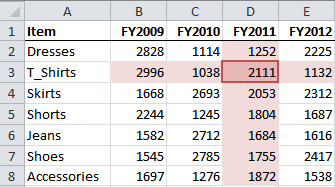
And let’s say I wanted to find the value for T-Shirts for FY2011; I could simply enter this formula:
=D2:D8 B3:E3
=2111
Obviously I could also enter =D3 but then I'd need to know that that was the cell reference, which is not usually the case when you're doing a lookup, so we’ll ignore that for now.
Notice how there are no brackets in the formula (you don’t need them to lookup a single cell), and there is a space between the two ranges?
This space is the ‘intersect operator’, and it instructs Excel to find the value in the cell at the intersection of the two ranges, which is D3.
You could also use this formula to return text, since there is only one cell at the intersection.
Intersection of Named Ranges
While the above example works, it’s a bit laborious to enter the cell ranges, and since this is a lazy lookup we need to make it quicker and easier to enter.
To do this I’ve set up the following named ranges for each column and row in my table:
FY_2009 =B2:B8
FY_2010 =C2:C8
FY_2011 =D2:D8
FY_2012 =E2:E8
Dresses =B2:E2
T_Shirts =B3:E3
And so on…
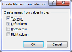
Tip: I set up all these named ranges in just a few steps:
- Highlight the table, including headers
- CTRL+SHIFT+F3 to create named ranges from selection. This opens the following dialog box:
- Click OK
Now I have my named ranges set up I can write the formula above like this:
=T_Shirts FY_2011
=2111
Again, no brackets, just a space between the two names. I think you’ll agree this now meets the ‘lazy’ requirement quite nicely.
SUM Multiple Cells
What say you wanted to SUM FY2010 and FY2011 for Skirts and Shorts?
You could use this formula:
=SUM(FY_2010:FY_2011 Skirts:Shorts)
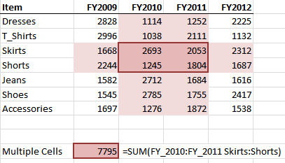
Notes:
- Because there are multiple cells at the intersection you must wrap your named ranges in a SUM function, or AVERAGE, MIN, MAX etc.
- Also, you cannot return text where there are multiple cells at the intersection.
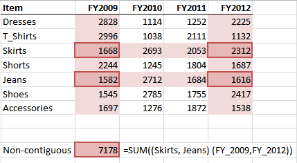
Non-contiguous Ranges
If you want to return the SUM of non-contiguous ranges simply group each set of rows and each set of columns together inside brackets like this:
Make it Interactive
Now for the ultimate in laziness, get someone else to build the formula by giving them data validation lists and use the INDIRECT function to build the formula on the fly.
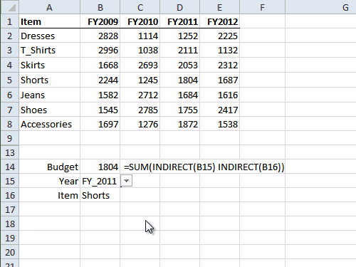
Note: the figures used in this example are fictional (I created them using the RANDBETWEEN function); I would never accept a reduction in my clothing budget year on year. 😉
Thanks to Kathy for sharing the Intersect Operator with us.
Kathy Carmel lives in Santa Barbara, California.
"I work with various forms of health care data, program in SAS and use Excel for deliverables and transitioning data to non-programmers. I have been using Excel for many years, mostly at a relatively basic level, but am now writing macros to do more of the analysis in Excel."
Vote for Kathy
If you’d like to vote for Kathy's tip (in X-factor voting style) use the buttons below to Like this on Facebook, Tweet about it on Twitter, +1 it on Google, Share it on LinkedIn, or leave a comment to thank Kathy for taking the time to share this tip….or all of the above 🙂

Thanks Mynda and Kathy.
I believe ‘lazy’ users of Excel are the best users… as they keep trying to find a faster, better way of doing things, push limits of Excel…
It is a GREAT thing that these ‘lazy’ people are NOT lazy when it comes to sharing their findings… so thanks all those out there who love to share.
🙂 glad you agree.
This tip is brilliant. I had never come across the use of the space to select the intersection of cells.
I had one issue when preparing the named ranges: Excel tagged an underscore to the end of the Year values so the Indirect wouldn’t work. I changed the values from “FY2009” (which became “FY2009_”) to “FY_2009” and then derived the range names. Perfect!
Glad you liked it, Dave 🙂
Quick question: when you used CTRL+SHIFT+F3 to create named ranges from selection, I assume you were working on a standard keyboard. I use a laptop. Would I also need to use the FN key to select the F3 function?
Great tip!!! Keep them coming!
Thank you
mks
Hi Marian,
Yes, you would have to press FN as well if you don’t have dedicated function keys on your keyboard.
Mynda
Kathy, Very Nice & Useful Tips,
With Thanks and Regards,
Chandru Parthiban
Hi Mynda,
I use intersection of named ranges across multiple workbooks.
Each workbook being identical in structure.
I am hoping to find most efficient syntax for formula like:
Book1.xlsx! Qtr1 Sales + Book2.xlsx! Qtr1 Sales + Book3.xlsx! Qtr1 Sales
But seems like I have to type:
Book1.xlsx!Qtr1 Book1.xlsx!Sales + Book2…….
Is there a more efficient syntax than above ?
Many Thanks,
Gordon.
Hi Gordon,
I’m not sure what the intersection of named ranges has to do with your formula as it looks like you want to sum/add ranges. If so, you can use a formula like this:
=SUM([Book1.xls]’Qtr 1 Sales’!$B$2:$B$20,[Book2.xls]’Qtr 1 Sales’!$B$2:$B$20,[Book3.xls]’Qtr 1 Sales’!$B$2:$B$20)
Note: Substitute $B$2:$B$20 for your named range if desired.
I hope that helps. I’m not aware of any simpler formulas.
Kind regards,
Mynda.
excellent !!
🙂 thanks, Khalid.
understood and thanks for nice tip.
You’re welcome, Khurram 🙂
Dear Mynda,
I tried the above with exact details as shown above and made the data validation lists and put in the formula =SUM(INDIRECT(B15) INDIRECT(B16)) result I am getting is null error.
You have two hidden rows (10,11) in your example above. Is there anything there?
Kindly advise
Regards. Subash
P.S. All the comments below were posted on my birthday last year. -:)
Hi Subash,
What post are you referring to?
What example and what file?
Cheers,
CarloE
Hi Carlo,
“Make it Interactive” in
“Excel Factor 15 The Lazy Lookup”
Rgds,
Subash
Hi Subash,
Believe me nothing is hidden in there. lol.
Now, I also tried to walk-through this and we got the same error.
By luck however I followed the named range to the letter: FY_2009, FY_2010, FY_2011, FY_2012.
I surmise you also skipped the underscore(“_”)because we are both ‘lazy’? lol.
Cheers,
CarloE
PS: If this don’t work, don’t ask me again. Ask Mynda. 😛
Hi Carlo,
It did work, but in my file the automated name range was FY2009_ and not FY_2009. Lazy eh !
Thanks very much.
Regards.
Subash
Hi Subash,
I’m the only one who’s lazy. 😉
Anyway, but you still have the underscore.
Cheers,
CarloE
Carlo,
Hi, we all are lazy that is where Excel comes in……
Keep up the good work of sharing knowledge my brother.
Regards,
Subash
amazing tip, wasn’t aware of the Intersect operator. And again: another lovely use (or lazily use?) of named ranges… Thanks for this tip…
🙂 Cheers, Phil.
THANK YOU VERY MUCH
You’re welcome, Ravi 🙂
i’m agree with you … “there’s nothing wrong with being lazy” … on the contrary 🙂
nice article, for me particularly interesting the section “Non-contiguous Ranges”
regards
r
Thank you, r!