• Skip to main content
  • Skip to header right navigation
  • Skip to site footer

My Online Training Hub

Learn Dashboards, Excel, Power BI, Power Query, Power Pivot

  • Courses
  • Pricing
    • SALE 20% Off All Courses
    • Free Courses
    • Power BI Course
    • Excel Power Query Course
    • Power Pivot and DAX Course
    • Excel Dashboard Course
    • Excel PivotTable Course โ€“ Quick Start
    • Advanced Excel Formulas Course
    • Excel Expert Advanced Excel Training
    • Excel Tables Course
    • Excel, Word, Outlook
    • Financial Modelling Course
    • Excel PivotTable Course
    • Excel for Customer Service Professionals
    • Multi-User Pricing
  • Resources
    • Free Downloads
    • Excel Functions Explained
    • Excel Formulas
    • Excel Add-ins
    • IF Function
      • Excel IF Statement Explained
      • Excel IF AND OR Functions
      • IF Formula Builder
    • Time & Dates in Excel
      • Excel Date & Time
      • Calculating Time in Excel
      • Excel Time Calculation Tricks
      • Excel Date and Time Formatting
    • Excel Keyboard Shortcuts
    • Excel Custom Number Format Guide
    • Pivot Tables Guide
    • VLOOKUP Guide
    • ALT Codes
    • Excel VBA & Macros
    • Excel User Forms
    • VBA String Functions
  • Members
    • Login
    • Logout
    • Password Reset
  • Blog
  • Excel Webinars
  • Excel Forum
    • Register as Forum Member

Excel Factor 16 Dynamic Lookup

You are here: Home / Excel Formulas / Excel Factor 16 Dynamic Lookup
Excel Factor 16 Dynamic Lookup
September 22, 2012 by Mynda Treacy
This Excel Factor tutorial was sent in by Bryon Smedley of Bristol, Tennessee.

Words by Bryon Smedley.

Enter your email address below to download the sample workbook.


By submitting your email address you agree that we can email you our Excel newsletter.
Please enter a valid email address.

Download the Excel Workbook and follow along. Note: This is a .xlsx file. Please ensure your browser doesn't change the file extension on download.

VLOOKUP is great for returning information from a database, but one of the limitations is that the return information is static.

What if the user wishes to look for certain data one day but different data another day?ย  This would require either two different sets of VLOOKUP functions or the functions would need to be reprogrammed.

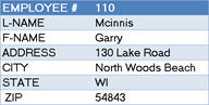
In the database below, the user would wish to return address information in one scenario, but return financial information in another scenario.

Suppose there are times when the user requires a mixture of the two; that would require a third set of VLOOKUP functions.ย This could become an ever evolving set of work.

ORIGINAL DATABASE

Excel Dynamic Lookup

ADDRESS INFORMATION

Excel Dynamic Lookup

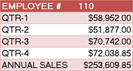
FINANCIAL INFORMATION
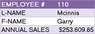
Excel Dynamic Lookup

MIXED INFORMATION

Excel Dynamic Lookup

Here comes MATCH to the rescue!!!

The MATCH function's job is to return the relative position of data within a defined array.

The syntax for the MATCH function is:

=MATCH(Lookup_value,Lookup_array,Match_type)
  • Lookup_value - The value that you want to find in the list of data. This argument can be a number, text, logical value, or a cell reference.
  • Lookup_array - The range of cells being searched.
  • Match_type (optional) Tells Excel how to match the Lookup_value with values in the Lookup_array. Choices: -1, 0, or 1. The default value for this argument is 1.
    • If the Match_type = 1 or is omitted: MATCH finds the largest value that is less than or equal to the Lookup_value. The Lookup_array data must be sorted in ascending order.
    • If the match_type = 0: MATCH finds the first value that is exactly equal to the Lookup_value. The Lookup_array data can be sorted in any order.
    • If the Match_type = -1: MATCH finds the smallest value that is greater than or equal to the Lookup_value. The Lookup_array data must be sorted in descending order.

If we wish to give the user the ability to dynamically select which fields of interest to return information from, the MATCH function can examine the category for each row (or column) and use it to calculate the position of that choice in the database.

That position number can then be used for the VLOOKUP Col_Index_Num variable.

*** Remember - VLOOKUP has the following syntax: ***

Excel VLOOKUP

Letโ€™s look at a VLOOKUP from the static ADDRESS INFORMATION table (FYI: The above database which occupies range $A$5:$L$29 has been given a NAMED RANGE of โ€œDatabase1โ€)

Excel VLOOKUP

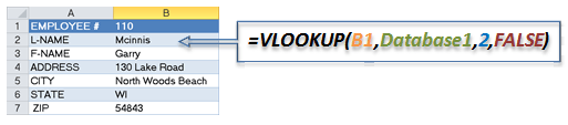
The "2" in the third variable position is telling us to return data from the 2nd relative column position from within the table (in this case, Column "B").

We can calculate that position with the following MATCH function (FYI: The databaseโ€™s header row which occupies range $A$4:$L$4 contains all of the category names and has been given a NAMED RANGE of "Categories")

=MATCH(A2,Categories,0)

If we execute this function by itself, it would return "2" as an answer, since "L-Name" exists in the 2nd column of the database.

Now we'll substitute the original "2" in the Col_Index_Num variable with the MATCH function:

=VLOOKUP(B1,Database1,MATCH(A2,Categories,0),FALSE)

*** IMPORTANT ***

The categories that the user types in Column "A" (in the above example) MUST match the names used in the database header row.

Letโ€™s add some pizzazz to this process

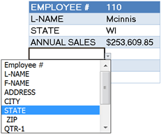
Since a requirement of the MATCH function is we use the same naming convention as the database, and the database contains all of the names, letโ€™s use those names in a dropdown list so the user can select items with greater ease and precision.

This can be accomplished by use of the Data Validation tool.

Excel VLOOKUP

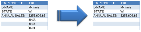
If we define a report area large enough to display all of a recordโ€™s information (accommodate the maximum number of return items), what happens when a user does not use all of the slots?

Any place a category is not defined, a โ€œ#N/Aโ€ error message will appear.ย  By placing all of the above VLOOKUP logic inside of an IFERROR function, we can suppress the โ€œ#N/Aโ€ error messages.

The blanks are generated by means of two double quotation marks placed side by side (no space between them).

Excel VLOOKUP

=IFERROR(VLOOKUP(B1,Database1,MATCH(A2,Categories,0),FALSE),"")

BONUS TRICK

If your dataset had non-user friendly headers, you could get fancy and have a table of official headings/user friendly headings and nest another VLOOKUP in the Lookup_Value variable position.

This would allow you to have understandable choices in your data validated dropdown list, but still find the correct category in the less friendly database headings.

Excel VLOOKUP

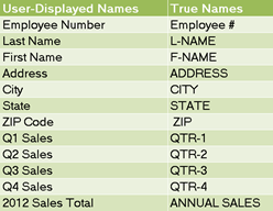
The table above was given the name "NewHeader"

=VLOOKUP(B1,Database1,MATCH(VLOOKUP(A2,NewHeader,2,False),Categories,0),FALSE)

Thanks again, Bryon for writing this tutorial and using color coding and loads of images to help us follow along. We appreciate you sharing your knowledge.

Bryon is from Bristol, Tennessee and has been teaching Excel since version 7 which was included with Office 95. He is currently a Technical Training Analyst for one of the largest coal companies in the world.ย  His key responsibility is to conduct all Microsoft Office training, but in addition he also serves as a technical consultant for any and all projects involving Microsoft Office applications.

Bryon says โ€œExcel is by far my favorite among all the Office applications due to the almost infinite number of situations it can be used.ย  There literally seems to be no end to its usefulness.

My favorite Excel tools are difficult to narrow down.ย  Without getting into third party add-ins, I would have to say PivotTables (especially with the addition of Slicers.ย  WOW!ย  Are those things awesome!!), the Text to Columns tool (what a time saver), and Macros.โ€

Vote for Bryon

If youโ€™d like to vote for Bryonโ€™s tip (in X-factor voting style) use the buttons below to Like this on Facebook, Tweet about it on Twitter, +1 it on Google, Share it on LinkedIn, or leave a comment to thank Bryon for taking the time to share his knowledgeโ€ฆ.or all of the above ๐Ÿ™‚

Excel Factor 16 Dynamic Lookup

More Excel_Factor Posts

Excel Factor Voting Roundup

Excel Factor Voting Roundup

Excel Factor 21 Hyperlink Triptych

Excel Factor 21 Hyperlink Triptych

Tips and tricks with hyperlinks to make them dynamically update as the selection in the sheet changes. Sample workbook available.
Excel Factor 20 Custom Number Format Disguise

Excel Factor 20 Custom Number Format Disguise

Excel Factor 19 Dynamic Dependent Data Validation

Excel Factor 19 Dynamic Dependent Data Validation

Excel Factor 18 Dynamic Hyperlinks and the Magic Hash

Excel Factor 18 Dynamic Hyperlinks and the Magic Hash

The Excel HYPERLINK function creates links to places inside or outside of your Excel file. I'll show you a shortcut for creating them that few people know.
Excel Factor 17 Lookup and Return Multiple Matches

Excel Factor 17 Lookup and Return Multiple Matches

Excel Factor 15 The Lazy Lookup

Excel Factor 15 The Lazy Lookup

Excel Factor 14 Interleave Data from Two Columns into One

Excel Factor 14 Interleave Data from Two Columns into One

Excel Factor 13 Handy Tips & Tricks

Excel Factor 13 Handy Tips & Tricks

Excel Factor 12 Secret EVALUATE Function

Excel Factor 12 Secret EVALUATE Function

More Vlookup Posts

vlookup in power query using list functions

VLOOKUP in Power Query Using List Functions

Use List functions to do VLOOKUPS in Power Query as an alternative to merging tables. Sample data and file available to download
VLOOKUP Multiple Values in Multiple Columns

VLOOKUP Multiple Values in Multiple Columns

Excel VLOOKUP Multiple Sheets

Excel VLOOKUP Multiple Sheets

Excel Factor 17 Lookup and Return Multiple Matches

Excel Factor 17 Lookup and Return Multiple Matches

VLOOKUP Multiple Criteria

VLOOKUP Multiple Criteria

Excel VLOOKUP Multiple Values

Excel VLOOKUP Multiple Values

Excel Wildcards in your SUMIF, COUNTIF and VLOOKUP

Excel Wildcards in your SUMIF, COUNTIF and VLOOKUP

Excel VLOOKUP with Dynamic Column Reference

Excel VLOOKUP with Dynamic Column Reference

Excel VLOOKUP with Dynamic Column Reference allows you to copy the formula across columns and have the column reference automatically update.
Excel VLOOKUP to the Left Using CHOOSE

Excel VLOOKUP to the Left Using CHOOSE

VLOOKUP to the left with this clever use of CHOOSE to trick Excel into looking up a column to the left.
hlookup function

Excel HLOOKUP Formulas Explained

How to use Excel HLOOKUP formula, including examples and workbook download.

More Excel Formulas Posts

top excel functions for data analysts

Top Excel Functions for Data Analysts

Must know Excel Functions for Data Analysts and what functions you donโ€™t have to waste time learning and why.
excel advanced formula environment

Excel Advanced Formula Environment

Excel Advanced Formula Environment is a long awaited, new improved way to write, name and store Excel formulas.
Pro Excel Formula Writing Tips

Pro Excel Formula Writing Tips

Must know Excel formula writing tips, tricks and tools to make you an Excel formula ninja, including a new formula editor.
excel shaping arrays

New Array Shaping Excel Functions

The Excel Shaping Array Functions makes it easier than ever to reshape arrays and ranges using these purpose built functions
excel nested if functions what not to do

Excel IF Formulas and What Not To Do

Excel IF formulas can get out of hand when you nest too many IFs. Not only do they become unwieldy theyโ€™re difficult for anyone to understand
excel image function

Excel IMAGE Function

The Excel IMAGE Function enables you to embed images in a cell using a formula. It supports BMP, JPG/JPEG, GIF, TIFF, PNG, ICO, and WEBP files

Excel VSTACK and HSTACK Functions

New Excel VSTACK and HSTACK functions makes combining arrays of cells easy and with some clever tricks we can extend their capabilities.
identify overlapping dates and times in excel

Identify overlapping dates and times in Excel

How to identify overlapping dates and times in Excel with a formula that checks a range of cells. Works with Dates and Times.
New Excel Text Functions

TEXTSPLIT, TEXTBEFORE and TEXTAFTER Functions

TEXTAFTER, TEXTBEFORE and TEXTSPLIT are exciting new Excel Text functions. Theyโ€™re fairly self-explanatory, however TEXTSPLIT has some cool features.

Top 10 Intermediate Excel Functions

Take your Excel skills to the next level with this top 10 intermediate Excel functions. These are must know functions for all Excel users.


Category: Excel FormulasTag: Excel_Factor, vlookup
Previous Post:Excel Factor 15 The Lazy LookupExcel Factor 15 The Lazy Lookup
Next Post:Excel Factor 17 Lookup and Return Multiple MatchesExcel Factor 17 Lookup and Return Multiple Matches

Reader Interactions

Comments

  1. Murari

    February 27, 2014 at 11:10 pm

    Dear Mynda, Your site is so helpful for learning so many skills. Thanks for proving help & support needed for day to day work life.

    I need a help from this forum. Let me explain what the problem.

    1. There are values in the column A, column B, column C, column D
    2. If the values matches from column A & C it will return either ‘1’ or ‘0’ depending on the match case and would be stored in column B
    3. Now, i need to fetch or extract values from column D if the match result is ‘1’ in the column B then store in the column F.

    Please help me how to do this task success.

    If any further clarifications needed with this matter, please let me know i can edit according to your reply.

    Reply
    • Catalin Bombea

      February 28, 2014 at 2:45 pm

      Hi Murari,
      Can you upload a sample workbook with your requirements? It will be a great help for us to undertand exactly your situation.
      You can use our Help Desk
      Thanks,
      Catalin

      Reply
  2. Mike M

    June 6, 2013 at 12:29 am

    Hi,
    I am trying to create a Data Table that has Dates such as July 1,2013, July 2,2013, ….. as the column headings the rows are filled with zip codes. I need to search the row data for a zip code match and return the column heading date. This is a scheduling data base that allows us to schedule work in the same area so some rows may be blank through out the data table.

    Reply
    • Mynda Treacy

      June 6, 2013 at 10:00 am

      Hi Mike,

      You could use this array formula:

      =INDEX(your row of dates,,MIN(IF(your table of data=your zip code,{1,2,3,4,5,6},"")))

      Entered with CTRL+SHIFT+ENTER because it’s an array formula, and where {1,2,3,4,5,6} represent the columns in your row of dates.

      e.g.:

      =INDEX(B1:G1,,MIN(IF(B2:G50=A1,{1,2,3,4,5,6},"")))

      If you get stuck please send me the file via the help desk.

      Kind regards,

      Mynda.

      Reply
  3. ron

    June 1, 2013 at 6:08 am

    I like the example worksheet.

    There are a couple of changes I would suggest
    1. on the lookup sheet create an identifiable single input field for employee number. I used B2

    2. change all references to employee number to point to that one input location rather than the individual table heading as is currently done in some.

    3. Is employee number the most logical way of selecting employees? I’m thinking a dropdown displaying all employee names, returning employee number may be easier for person doing the input.

    Reply
    • Mynda Treacy

      June 3, 2013 at 7:43 am

      Cheers, Ron. All great ideas to add a bit more functionality and adapt it to your needs and the way you work.

      Thanks for sharing ๐Ÿ™‚

      Mynda.

      Reply
  4. Mike

    February 14, 2013 at 8:43 am

    I like the concept of this one, the user can make their own report.

    Additionally, make ranges ‘Categories’ and ‘Database1’ dynamic with the offset and counta function to set the ranges, so added records and columns will be included within the search and results without any changes to existing formulas.

    Just found this site this evening – looks good!

    Reply
    • Mynda Treacy

      February 14, 2013 at 9:07 am

      Cheers, Mike. Thanks for sharing ๐Ÿ™‚

      Reply
  5. Raghu

    September 26, 2012 at 1:52 pm

    Hi ! Could you attach an excel work sheet for this. it would be easy to understand better while actually working out on an example.

    Reply
    • Mynda Treacy

      September 26, 2012 at 11:12 pm

      Hi Raghu,

      Here is the file from Bryon.

      Kind regards,

      Mynda.

      Reply

Leave a Reply Cancel reply

Your email address will not be published. Required fields are marked *

Current ye@r *

Leave this field empty

Sidebar

More results...

Course Sale

mynda treacy microsoft mvpHi, I'm Mynda Treacy and I run MOTH with my husband, Phil. Through our blog, webinars, YouTube channel and courses we hope we can help you learn Excel, Power Pivot and DAX, Power Query, Power BI, and Excel Dashboards.

Subscribe to Our Newsletter

Receive weekly tutorials on Excel, Power Query, Power Pivot, Power BI and More.

We respect your email privacy

Guides and Resources

  • Excel Keyboard Shortcuts
  • Excel Functions
  • Excel Formulas
  • Excel Custom Number Formatting
  • ALT Codes
  • Pivot Tables
  • VLOOKUP
  • VBA
  • Excel Userforms
  • Free Downloads

239 Excel Keyboard Shortcuts

Download Free PDF

Free Webinars

Excel Dashboards Webinar

Watch our free webinars and learn to create Interactive Dashboard Reports in Excel or Power BI

Click Here to Watch Now

Blog Categories

  • Excel
  • Excel Charts
  • Excel Dashboard
  • Excel Formulas
  • Excel PivotTables
  • Excel Shortcuts
  • Excel VBA
  • General Tips
  • Online Training
  • Outlook
  • Power Apps
  • Power Automate
  • Power BI
  • Power Pivot
  • Power Query
trustpilot excellent rating
 

Company

  • About My Online Training Hub
  • Disclosure Statement
  • Frequently Asked Questions
  • Guarantee
  • Privacy Policy
  • Terms & Conditions
  • Testimonials
  • Become an Affiliate

Support

  • Contact
  • Forum
  • Helpdesk – For Technical Issues

Copyright © 2023 · My Online Training Hub · All Rights Reserved

Microsoft and the Microsoft Office logo are trademarks or registered trademarks of Microsoft Corporation in the United States and/or other countries. Product names, logos, brands, and other trademarks featured or referred to within this website are the property of their respective trademark holders.