• Skip to main content
  • Skip to header right navigation
  • Skip to site footer

My Online Training Hub

Learn Dashboards, Excel, Power BI, Power Query, Power Pivot

  • Courses
  • Pricing
    • Free Courses
    • Power BI Course
    • Excel Power Query Course
    • Power Pivot and DAX Course
    • Excel Dashboard Course
    • Excel PivotTable Course – Quick Start
    • Advanced Excel Formulas Course
    • Excel Expert Advanced Excel Training
    • Excel Tables Course
    • Excel, Word, Outlook
    • Financial Modelling Course
    • Excel PivotTable Course
    • Excel for Customer Service Professionals
    • Excel for Operations Management Course
    • Excel for Decision Making Under Uncertainty Course
    • Excel for Finance Course
    • Excel Analysis ToolPak Course
    • Multi-User Pricing
  • Resources
    • Free Downloads
    • Excel Functions Explained
    • Excel Formulas
    • Excel Add-ins
    • IF Function
      • Excel IF Statement Explained
      • Excel IF AND OR Functions
      • IF Formula Builder
    • Time & Dates in Excel
      • Excel Date & Time
      • Calculating Time in Excel
      • Excel Time Calculation Tricks
      • Excel Date and Time Formatting
    • Excel Keyboard Shortcuts
    • Excel Custom Number Format Guide
    • Pivot Tables Guide
    • VLOOKUP Guide
    • ALT Codes
    • Excel VBA & Macros
    • Excel User Forms
    • VBA String Functions
  • Members
    • Login
  • Blog
  • Excel Webinars
  • Excel Forum
    • Register as Forum Member
  • Login

Excel Factor 14 Interleave Data from Two Columns into One

You are here: Home / Excel Formulas / Excel Factor 14 Interleave Data from Two Columns into One
Excel Factor 14 Interleave Data from Two Columns into One
September 12, 2012 by Mynda Treacy
This Excel Factor tutorial was sent in by Bryon Smedley of Bristol, Tennessee.

I have to admit, this problem doesn't come up often, but when it does, this is a very slick way to eliminate hours of retyping or copy/pasting.

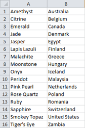
Suppose you have two columns of data and you want to create a third column of data generated from the first two.  The catch is we need to interleave the data from one column into the next.

Column “A” is a list of gemstones. Column “B” is a list of countries.

Excel INDIRECT function to merge two columns

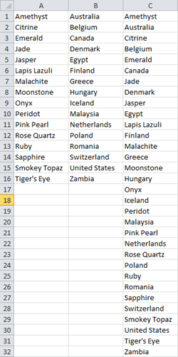
We need the resulting list to look like this:
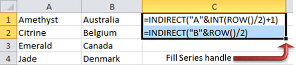
Excel INDIRECT function to combine two columns

In cell C1, type

=INDIRECT("A"&INT(ROW()/2)+1)

In cell C2, type

=INDIRECT("B"&ROW()/2)

After you have these two formulas in place, highlight BOTH formulas and then grab the fill series handle and pull down as far as needed to create a single column containing all of the combined data.

Excel INDIRECT function to merge two columns

Here’s how it works:

Cell C1 Formula

=INDIRECT("A"&INT(ROW()/2)+1)

Take the current row number, divide it by two, round it down to closest integer, add one, and concatenate an A in front of it.

Cell C2 Formula

=INDIRECT("B"&ROW()/2)

Take the current row number, divide it by two, and concatenate an B in front of it.

The result of both calculations is used by the INDIRECT function as an instruction of what do to; in this case, =A1 (show what is in A1), and =B1 (show what is in B1).

Thanks again, Bryon for writing this tutorial and using color coding to help us follow along. We appreciate you sharing your knowledge.

Bryon is from Bristol, Tennessee and has been teaching Excel since version 7 which was included with Office 95. He is currently a Technical Training Analyst for one of the largest coal companies in the world.  His key responsibility is to conduct all Microsoft Office training, but in addition he also serves as a technical consultant for any and all projects involving Microsoft Office applications. Bryon says “Excel is by far my favorite among all the Office applications due to the almost infinite number of situations it can be used.  There literally seems to be no end to its usefulness. My favorite Excel tools are difficult to narrow down.  Without getting into third party add-ins, I would have to say PivotTables (especially with the addition of Slicers.  WOW!  Are those things awesome!!), the Text to Columns tool (what a time saver), and Macros.”

Vote for Bryon

If you’d like to vote for Bryon’s tip (in X-factor voting style) use the buttons below to Like this on Facebook, Tweet about it on Twitter, +1 it on Google, Share it on LinkedIn, or leave a comment to thank Bryon for taking the time to share his knowledge….or all of the above 🙂

Excel Factor 14 Interleave Data from Two Columns into One
Mynda Treacy

Microsoft MVP logo

AUTHOR Mynda Treacy Co-Founder / Owner at My Online Training Hub

CIMA qualified Accountant with over 25 years experience in roles such as Global IT Financial Controller for investment banking firms Barclays Capital and NatWest Markets.

Mynda has been awarded Microsoft MVP status every year since 2014 for her expertise and contributions to educating people about Microsoft Excel.

Mynda teaches several courses here at MOTH including Excel Expert, Excel Dashboards, Power BI, Power Query and Power Pivot.

More Excel_Factor Posts

Excel Factor Voting Roundup

Excel Factor Voting Roundup

Excel Factor 21 Hyperlink Triptych

Excel Factor 21 Hyperlink Triptych

Tips and tricks with hyperlinks to make them dynamically update as the selection in the sheet changes. Sample workbook available.
Excel Factor 20 Custom Number Format Disguise

Excel Factor 20 Custom Number Format Disguise

Excel Factor 19 Dynamic Dependent Data Validation

Excel Factor 19 Dynamic Dependent Data Validation

Excel Factor 18 Dynamic Hyperlinks and the Magic Hash

Excel Factor 18 Dynamic Hyperlinks and the Magic Hash

The Excel HYPERLINK function creates links to places inside or outside of your Excel file. I'll show you a shortcut for creating them that few people know.
Excel Factor 17 Lookup and Return Multiple Matches

Excel Factor 17 Lookup and Return Multiple Matches

Excel Factor 16 Dynamic Lookup

Excel Factor 16 Dynamic Lookup

Excel Factor 15 The Lazy Lookup

Excel Factor 15 The Lazy Lookup

Excel Factor 13 Handy Tips & Tricks

Excel Factor 13 Handy Tips & Tricks

Excel Factor 12 Secret EVALUATE Function

Excel Factor 12 Secret EVALUATE Function

More Excel Formulas Posts

Summarize Months to Quarters

Excel Formulas to Summarise Monthly Data into Quarters

3 ways (good, better, best) to summarize monthly data into quarters using formulas. Lots of examples and sample file to download.
Excel BYROW and BYCOL Functions

Excel BYCOL and BYROW Functions

Excel BYCOL and BYROW functions fundamentally change the way we write formulas that calculate across columns and down rows.
python in excel natively

How to Use Python in Excel Natively

How to use Python in Excel natively using libraries like Pandas, NumPy, Matplotlib, Seaborn and more for analysis and spectacular charts!
excel dynamic named ranges

Excel Dynamic Named Ranges

Excel Dynamic Named Ranges update automatically to include new data in the ranges referenced in your formulas and PivotTables etc.
functions for financial modelling

Excel Functions for Financial Modeling

Top 23 must know Excel functions for Financial Modeling. Includes example Excel file and step by step instructions.
excel formula by example

Excel Formula by Example

Excel can now write a formula by example. Simply give it an example or two of the result and Excel will write the formula.
ai-aided excel formula editor

AI Aided Excel Formula Editor

Save time with this free AI Excel formula editor add-in that writes, edits, improves and interprets formulas for you!
top excel functions for data analysts

Top Excel Functions for Data Analysts

Must know Excel Functions for Data Analysts and what functions you don’t have to waste time learning and why.
excel advanced formula environment

Excel Labs (Formerly, Advanced Formula Environment)

Excel Labs is a long awaited, new improved way to write, name and store Excel formulas, including LAMBDAS with the help of AI.
Pro Excel Formula Writing Tips

Pro Excel Formula Writing Tips

Must know Excel formula writing tips, tricks and tools to make you an Excel formula ninja, including a new formula editor.


Category: Excel FormulasTag: Excel_Factor
Previous Post:Excel Factor 13 Handy Tips & TricksExcel Factor 13 Handy Tips & Tricks
Next Post:Excel Factor 15 The Lazy LookupExcel Factor 15 The Lazy Lookup

Reader Interactions

Comments

  1. Dario A

    April 3, 2020 at 11:19 pm

    if you have more than two elements to interleave, say 4, this worked for me =TRANSPOSE(INDIRECT(“A”&INT(ROW()/4)+1):INDIRECT(“D”&INT(ROW()/4)+1))

    Reply
    • Mynda Treacy

      April 4, 2020 at 10:01 am

      Thanks for sharing, Dario.

      Reply
  2. Minnesota Prof

    June 19, 2019 at 5:07 am

    THanks for this…I had to create tables for an academic paper from figures in statistical output. This trick.worked really well and saved me hours of labor. Thanks for this amazningly valuable tip!

    Reply
  3. Eric

    March 24, 2018 at 5:31 am

    Thanks, it works!
    I had to remove blank cells first, but it saved me a lot of time and it is very simple.

    Reply
    • Mynda Treacy

      March 25, 2018 at 11:03 am

      Glad you found it useful, Eric.

      Reply
  4. Dylan Chouinard

    March 21, 2018 at 11:07 am

    Hey all,

    I’m struggling with copying down the series of cell formulas – when I click and drag, it only pulls down the very first cell’s formula, not the ones underneath (I’m trying to interleave three columns into one over 2,900+ cells). Any shortcuts or tips to ensure that all three cells with different formulas are dragged down together in sequence?

    Thanks,
    Dylan

    Reply
    • Catalin Bombea

      March 24, 2018 at 2:22 am

      Hi Dylan,
      Hard to visualize how the data looks and what are you trying to do.
      Can you please upload a sample file with descriptions of what you want to do? Use our forum to create a new topic and upload the file, we will gladly help you, if it’s possible what you want.
      Regards
      Catalin

      Reply
  5. Paul Castle

    May 25, 2017 at 5:56 am

    Doesn’t work if one column is for a date, I’m afraid, and you get ‘40878’ instead of ’01/12/2011′. But I’m sure this’ll come in for something else.

    Reply
    • Mynda Treacy

      May 25, 2017 at 8:58 pm

      Hi Paul,

      That’s correct, just format the cell containing 40878 as a date and you’ll see it’s 1/12/2011. It’s just that the formula returns the date serial number, which is how Excel stores dates.

      You can read more about how Excel handles dates and time here.

      Mynda

      Reply
  6. Roni

    April 19, 2013 at 7:34 am

    What if I have data like this:
    Jan Feb Mar
    0.88 0.50 0.39
    0.86 0.50 0.36
    0.86 0.46 0.39
    0.79 0.43 0.39
    0.74 0.40 0.32
    0.74 0.43 0.35
    0.72 0.46 0.35
    0.75 0.46 0.36
    0.76 0.43 0.38
    0.75 0.50 0.42

    but want it arranged like this:
    Jan
    0.88
    0.86
    0.86
    0.79
    0.74
    0.74
    0.72
    0.75
    0.76
    0.75
    Feb
    0.5
    0.5
    0.46
    0.43
    0.4
    0.43
    0.46
    0.46
    0.43
    0.5

    etc.
    I get data like this all the time for each month and have to do it manually.

    Grateful for any help at all.
    Thanks!
    Roni

    Reply
    • Carlo Estopia

      April 19, 2013 at 1:33 pm

      Hi Roni,

      You know what? I don’t have a slick solution for this one.
      It could be a two-step solution.

      So say hello for me here: HELP DESK ; that is,
      if you want the solution anyway.

      By the way, the idea is like this:
      NOTE:Data is at A1:C7
      formula starts in A8

      Jan	Feb	Mar
      1	2	3
      4	5	6
      7	8	9
      0	a	b
      d	e	f
      
      
      =IF(ROW()<=13,INDIRECT("A"&ROW()-7),IF(ROW()<=19,INDIRECT("B"&ROW()-13),IF(ROW()<=25,INDIRECT("C"&ROW()-19))))
      

      You can then get the handle and drag as far as necessary.

      Cheers,

      CarloE

      Reply
  7. Roni

    November 13, 2012 at 3:32 am

    Well explained Byron. Thanks for sharing! Understand perfectly.

    Reply
  8. DJ Sachs

    September 12, 2012 at 11:16 pm

    This solution is sensitive to which row is the first row of data. The example above starts in Row 1. If the starting row isn’t Row 1 (i.e., if Row 1 contains column headings like “Gem” and “Country”), one of the formulas needs to be changed (depending on whether the first row is odd [“A” formula needs to be changed] or even [“B” formula needs to be changed]). Also, the INT function needs to be added to the “B” formula if the first row of data isn’t Row 1.

    if Starting Row is: Formula needed

    Row 1 "A" formula	=INDIRECT("A"&INT(ROW()/2)+1)
    Row 1 "B" formula	=INDIRECT("B"&INT(ROW()/2))
    Row 2 "A" formula	=INDIRECT("A"&INT(ROW()/2)+1)
    Row 2 "B" formula	=INDIRECT("B"&INT(ROW()/2)+1)
    Row 3 "A" formula	=INDIRECT("A"&INT(ROW()/2)+2)
    Row 3 "B" formula	=INDIRECT("B"&INT(ROW()/2)+1)
    Reply
    • Mynda Treacy

      September 12, 2012 at 11:22 pm

      True. Thanks for sharing, DJ Sachs 🙂

      Reply
      • aaron

        January 31, 2013 at 7:28 am

        What about if you are starting in row 6?

        I get the idea that you need to change one of the two formulas depending on where your data begins. I don’t understand what parts of the formula to change to make it work with the appropriate row.

        What are the ‘fixed’ and variable parts of the formula?

        PS. this is the only good tutorial on this issue I could find. It was hard to find the correct words to describe and google the problem. Thank you!!

        Reply
        • Carlo Estopia

          January 31, 2013 at 2:31 pm

          Dear Aaron,

          The variable part is merely the + 1 part. that’s all. simply replace it to get A1 or B1 respectively in the INT FUNCTION PART. Also follow the formula in A when you want to improvise.
          NOTE:INT will take away decimal.

          For example: if you want to start in 6 and 7. Your formula should be

           at row 6 =INDIRECT("A"&INT(ROW()/2-2)  
          and at row 7 = INDIRECT("B"&INT(ROW()/2-2)
          simple explanation:
          row6/2 = 3.. how much will you need to get 1? so? -2 .
          row7/2 = 3.5 Disregard the .5 and you get 3. how much will you need to get1? hence - 2. 

          Detailed analysis:

          Put this formula: INDIRECT(“A”&INT(ROW()/2)+1)) in E1
          isolate INT(ROW())/2 in G1 NOTE: no +1 and the /2 is outside the INT Function for emphasis

          Get the handles and drag the formulas both as far as row 7.

          you’ll see at first that it will look like this:
          E1 ……………………….. G1
          amethyst ———————–.5
          diamond ———————— 1
          diamond ———————– 1.5
          jam ———————–2
          jam ———————–2.5
          okay ———————–3
          okay ———————– 3.5
          NOTE: to convert back the values in col G to its actual result. just remove the .5’s (do not round off) and +1.
          so….

           ACTUAL VALUES IN THE INT FUNCTION PART ( .5 = 1, 1=2, 1.5 =2, 2 =3, 2.5 =3 , 3 = 4, 3.5 = 4) 

          hence the result in E1

          you will notice that G1 is in the multiple of .5’s. Note that INT Function takes away any decimal out of a number.
          However, we put outside the /2 out of the INT Function and no + 1. hence if we’re in row 1.
          1/2 = .5 … row 2; 2/2 = 1 etc.

          Now in E1.. you will notice that only Amethyst is not repeated. The rest are repeated twice.
          So the question: Why? If we put back the 2 inside the int function and put back the +1 inside the int function.
          It would have looked like this INT(current row(i.e. 1)/2 + 1) = 1 or INT(1.5) = 1.
          in row 2, INT(current row(2)/2 +1) = 2 or INT(2) = 2
          in row 3, INT(current row(3)/2 +1) = 2.5 or INT(2.5) = 2.. NOTE 2 and 3 are the same results
          So if you put at row 1 INdirect(“A” & INT(ROW()/2+1)) in row 1. it simply means =A1 or amethyst
          at row 2 Indirect(“A” & INTROW()/2+1)) in row 2. it simply means =A2 or diamond
          at row 3 Indirect(“A” & INTROW()/2+1)) in row 2. it simply means =A2 or diamond
          etc… as the illustration above shows.

          Now going back to your question, To put Amethyst in row 2… you simply ask yourself: What should I do with the formula to get the result of A1. It’s simple just add + 0… going back in the actual values highlighted above. INT(ROW/2+1) at row 2 will result to 1 … so replace + 1 and put 0 and you will get only 1 :A1.
          if in row 3, INT(ROW3/2) = 1 (.5 is taken away) ergo it is still + 0 at row 3 INT(ROW/2+0).
          if in row 4, INT(ROW4/2) = 2 ergo -1 this time to get A1 INT(ROW()/2-1).

          now how about in B? the concept is still simple. to get Australia where you want it. just follow the explanation we have above. Just get INT FUNCTION PART to 1; hence, if you want Australia in row 3… just think: INT(row 3/2) = 1 (.5 taken away) do you still want to add? of course not because you have a 1 already.

          I actually have a headache today but this is an interesting topic.

          Cheers,

          CarloE

          Reply
  9. saran

    September 12, 2012 at 1:43 pm

    +1 to Bryon.. well explained..

    I would solve this prob in different way..

    1. Copy Column A in Column C
    2. Copy Column B in Column C below A data.
    3. Type 1 in Cell D1, 3 in Cell D2 and drag the numbers till A column data ends
    4. Type 2 in Cell D17 (above), 4 in Cell D18 and drag the numbers till B column data ends
    5. Simply, sort the Column D from smallest to largest by selecting Column C & D
    6. Thant’s all !! Column C data is our solution

    I explained the solution to the guys, who don’t want to go for formulas.

    Please note that this is only alternative way of solving.. Bryon’s indirect formula way is ultimate.

    Regards,
    Saran

    Reply
    • Mynda Treacy

      September 12, 2012 at 1:55 pm

      Cheers, Saran. Great alternative.

      Reply
      • saran

        September 12, 2012 at 1:58 pm

        Cheers.. Mynda

        Reply
  10. Ravi Xavier

    September 12, 2012 at 1:37 pm

    Thank you very much this is very easy to understand indeed.

    Reply
    • Mynda Treacy

      September 12, 2012 at 1:41 pm

      Cheers, Ravi 🙂

      Reply

Leave a Reply Cancel reply

Your email address will not be published. Required fields are marked *

Current ye@r *

Leave this field empty

Sidebar

More results...

Popular Content

  • 10 Common Excel Mistakes to Avoid
  • Top Excel Functions for Data Analysts
  • Secrets to Building Excel Dashboards in Less Than 15 Minutes
  • Pro Excel Formula Writing Tips
  • Hidden Excel Double-Click Shortcuts
  • Top 10 Intermediate Excel Functions
  • 5 Pro Excel Dashboard Design Tips
  • 5 Excel SUM Function Tricks
  • 239 Excel Keyboard Shortcuts

100 Excel Tips and Tricks eBook

Download Free Tips & Tricks

239 Excel Keyboard Shortcuts

Download Free PDF

mynda treacy microsoft mvpHi, I'm Mynda Treacy and I run MOTH with my husband, Phil. Through our blog, webinars, YouTube channel and courses we hope we can help you learn Excel, Power Pivot and DAX, Power Query, Power BI, and Excel Dashboards.

Blog Categories

  • Excel
  • Excel Charts
  • Excel Dashboard
  • Excel Formulas
  • Excel Office Scripts
  • Excel PivotTables
  • Excel Shortcuts
  • Excel VBA
  • General Tips
  • Online Training
  • Outlook
  • Power Apps
  • Power Automate
  • Power BI
  • Power Pivot
  • Power Query
microsoft mvp logo
trustpilot excellent rating
Secured by Sucuri Badge
MyOnlineTrainingHub on YouTube Mynda Treacy on Linked In Mynda Treacy on Instagram Mynda Treacy on Twitter Mynda Treacy on Pinterest MyOnlineTrainingHub on Facebook

Sign up to our newsletter and join over 400,000
others who learn Excel and Power BI with us.


Company

  • About My Online Training Hub
  • Disclosure Statement
  • Frequently Asked Questions
  • Guarantee
  • Privacy Policy
  • Terms & Conditions
  • Testimonials
  • Become an Affiliate
  • Sponsor Our Newsletter

Support

  • Contact
  • Forum
  • Helpdesk – For Technical Issues

Copyright © 2023 · My Online Training Hub · All Rights Reserved. Microsoft and the Microsoft Office logo are trademarks or registered trademarks of Microsoft Corporation in the United States and/or other countries. Product names, logos, brands, and other trademarks featured or referred to within this website are the property of their respective trademark holders.

Download A Free Copy of 100 Excel Tips & Tricks

excel tips and tricks ebook

We respect your privacy. We won’t spam you.

x