• Skip to main content
  • Skip to header right navigation
  • Skip to site footer

My Online Training Hub

Learn Dashboards, Excel, Power BI, Power Query, Power Pivot

  • Courses
  • Pricing
    • Free Courses
    • Power BI Course
    • Excel Power Query Course
    • Power Pivot and DAX Course
    • Excel Dashboard Course
    • Excel PivotTable Course – Quick Start
    • Advanced Excel Formulas Course
    • Excel Expert Advanced Excel Training
    • Excel Tables Course
    • Excel, Word, Outlook
    • Financial Modelling Course
    • Excel PivotTable Course
    • Excel for Customer Service Professionals
    • Excel for Operations Management Course
    • Excel for Decision Making Under Uncertainty Course
    • Excel for Finance Course
    • Excel Analysis ToolPak Course
    • Multi-User Pricing
  • Resources
    • Free Downloads
    • Excel Functions Explained
    • Excel Formulas
    • Excel Add-ins
    • IF Function
      • Excel IF Statement Explained
      • Excel IF AND OR Functions
      • IF Formula Builder
    • Time & Dates in Excel
      • Excel Date & Time
      • Calculating Time in Excel
      • Excel Time Calculation Tricks
      • Excel Date and Time Formatting
    • Excel Keyboard Shortcuts
    • Excel Custom Number Format Guide
    • Pivot Tables Guide
    • VLOOKUP Guide
    • ALT Codes
    • Excel VBA & Macros
    • Excel User Forms
    • VBA String Functions
  • Members
    • Login
  • Blog
  • Excel Webinars
  • Excel Forum
    • Register as Forum Member
  • Login

INDEX MATCH With a Twist

You are here: Home / Excel Formulas / INDEX MATCH With a Twist
INDEX MATCH With a Twist
January 12, 2012 by Mynda Treacy

My Toughest Excel Challenge So Far!

Recently a member contacted me with a VLOOKUP question, but when I further understood the requirements it became a challenge I’d never come across before.

This pushed me to my Excel limits and I have to be honest…I nearly gave up twice! By giving up I mean I was going to settle for a work-around solution instead.

The Challenge

Christy wanted to find the last value in a row for a specific part number using a table of data in Sheet1 like this:

Index Match Formula

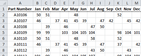
Notice how some rows don’t have a value in every cell? This is what makes this challenge unique.

You see Christy wanted to find the value for say, part A10106, for the month of June, but if June didn’t have a value then find the value for the previous month, and if May didn’t have a value then go to the previous month and so on.

And it wasn’t just one part, it was over 2000 parts and for every month of the year.

Not being one to shy away from a challenge I persisted, and this is my formula (Note: The table above was on Sheet1 and my formula is on Sheet2):

=IFERROR(INDEX(INDIRECT("Sheet1!"&ADDRESS(MATCH(A4, Sheet1!$A:$A,0),1,1)&":"&ADDRESS(MATCH(A4, Sheet1!$A:$A,0),MATCH(B3, Sheet1!$1:$1,0),1)),MATCH(9.99999999999999E+307,INDIRECT("Sheet1!" &ADDRESS(MATCH(A4, Sheet1!$A:$A,0),1,1)&":"&ADDRESS(MATCH(A4, Sheet1!$A:$A,0),MATCH(B3, Sheet1!$1:$1,0),1)))),0)

Phew. I’m not ashamed to say that I cheered out loud when I cracked this one.

Find Last Value in a Range

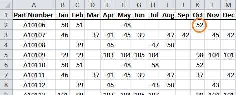
The first part of the challenge was to find the last value in each row.

We can use an INDEX and MATCH formula like this to find the last value in row 2:

=INDEX(Sheet1!A2:M2,MATCH(9.99999999999999E+307,Sheet1!A2:M2))

=52

Index Match Formula

But I need to find the last value for each month and for that I need the range A2:M2 to change for each month I look up, and for each part.

So that for Part Number A10106 for the month of June I look up the range Sheet1!A2:G2 and for the month of August I look up Sheet1!A2:I2, and so on.

To do this I need to replace the range Sheet1!A2:M2 with some functions that will dynamically update when I change the month and the Part Number, and for this I used INDIRECT, MATCH and ADDRESS.

Dynamic Range using INDIRECT, MATCH and ADDRESS

So my formula went from this:

=INDEX(Sheet1!A2:M2,MATCH(9.99999999999999E+307,Sheet1!A2:M2))

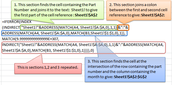
To this by replacing the ranges Sheet1!A2:M2 with the sections in blue:

=IFERROR(INDEX(INDIRECT("Sheet1!"&ADDRESS(MATCH(A4, Sheet1!$A:$A,0),1,1)&":"&ADDRESS(MATCH(A4, Sheet1!$A:$A,0),MATCH(B3, Sheet1!$1:$1,0),1)),MATCH(9.99999999999999E+307,INDIRECT("Sheet1!" &ADDRESS(MATCH(A4, Sheet1!$A:$A,0),1,1)&":"&ADDRESS(MATCH(A4, Sheet1!$A:$A,0),MATCH(B3, Sheet1!$1:$1,0),1)))),0)

Note: cell A4 contains the part number and B3 contains the month I want to look up.

The INDIRECT function returns a reference specified by a text string.

In this case the text string is generated using the MATCH function and I've used the ampersand to join components of the text string together.

The ADDRESS function obtains the address of a cell or range of cells. For example, ADDRESS(1,2) returns $A$2.

Index Match Functions

IFERROR - The Icing on the Top

And finally, if Excel couldn’t find the part number in the table I used the IFERROR function to enter a zero.

Download the Workbook

Enter your email address below to download the sample workbook.


By submitting your email address you agree that we can email you our Excel newsletter.
Please enter a valid email address.

If you would like a more in-depth understanding of this formula why not download the workbook and reverse engineer the formula, or use the Evaluate Formula tool to step through the formula and watch as each part evaluates.

You’ll find the evaluate tool on the Formulas tab of the Ribbon in the Formula Auditing group.

Feedback

I’d love to know if you have a simpler way to tackle this challenge. Please post your solution below in the comments for us all to share.

INDEX MATCH With a Twist
Mynda Treacy

Microsoft MVP logo

AUTHOR Mynda Treacy Co-Founder / Owner at My Online Training Hub

CIMA qualified Accountant with over 25 years experience in roles such as Global IT Financial Controller for investment banking firms Barclays Capital and NatWest Markets.

Mynda has been awarded Microsoft MVP status every year since 2014 for her expertise and contributions to educating people about Microsoft Excel.

Mynda teaches several courses here at MOTH including Excel Expert, Excel Dashboards, Power BI, Power Query and Power Pivot.

More Excel Formulas Posts

Summarize Months to Quarters

Excel Formulas to Summarise Monthly Data into Quarters

3 ways (good, better, best) to summarize monthly data into quarters using formulas. Lots of examples and sample file to download.
Excel BYROW and BYCOL Functions

Excel BYCOL and BYROW Functions

Excel BYCOL and BYROW functions fundamentally change the way we write formulas that calculate across columns and down rows.
python in excel natively

How to Use Python in Excel Natively

How to use Python in Excel natively using libraries like Pandas, NumPy, Matplotlib, Seaborn and more for analysis and spectacular charts!
excel dynamic named ranges

Excel Dynamic Named Ranges

Excel Dynamic Named Ranges update automatically to include new data in the ranges referenced in your formulas and PivotTables etc.
functions for financial modelling

Excel Functions for Financial Modeling

Top 23 must know Excel functions for Financial Modeling. Includes example Excel file and step by step instructions.
excel formula by example

Excel Formula by Example

Excel can now write a formula by example. Simply give it an example or two of the result and Excel will write the formula.
ai-aided excel formula editor

AI Aided Excel Formula Editor

Save time with this free AI Excel formula editor add-in that writes, edits, improves and interprets formulas for you!
top excel functions for data analysts

Top Excel Functions for Data Analysts

Must know Excel Functions for Data Analysts and what functions you don’t have to waste time learning and why.
excel advanced formula environment

Excel Labs (Formerly, Advanced Formula Environment)

Excel Labs is a long awaited, new improved way to write, name and store Excel formulas, including LAMBDAS with the help of AI.
Pro Excel Formula Writing Tips

Pro Excel Formula Writing Tips

Must know Excel formula writing tips, tricks and tools to make you an Excel formula ninja, including a new formula editor.


Category: Excel Formulas
Previous Post:Excel INDIRECT FunctionExcel INDIRECT Function
Next Post:ROUNDUP and ROUNDDOWN with a TwistROUNDUP and ROUNDDOWN with a Twist

Reader Interactions

Comments

  1. Howard Silcock

    November 24, 2019 at 10:59 pm

    I’ve only just seen this post and decided to have a go at doing it and see if dynamic arrays might help. Is the following formula simpler?
    =OFFSET(Sheet1!A1, MATCH(A4,part_number,0),
    MAX(IFERROR(MATCH(“?*” & “_” & SEQUENCE(MATCH(B3, months,0)),
    TRANSPOSE(OFFSET(Sheet1!A1,MATCH(A4,part_number,0),1,1,MATCH(B3, months,0))) & “_”
    & SEQUENCE(MATCH(B3, months,0)), 0), 0)))

    I have attached the original workbook to this post in the forum with my formula added on Sheet 2, together with another workbook that explains a technique I used – not sure if this is known. The basic idea is to extend the MATCH function so that it instead of returning just the first index where a match occurs, you return an array listing all the indexes where a match occurs.

    Reply
    • Mynda Treacy

      November 25, 2019 at 8:51 am

      Nice use of Dynamic Arrays, Howard! I’m not sue it’s much simpler, but it’s better because we don’t need INDIRECT. Thanks for sharing 🙂

      Reply
  2. Kthom019

    March 12, 2017 at 2:14 am

    I really need assistance with date formatting from numbers (20170227) or text (02-27-2017). My data is pulled with either formats, from which I need to convert to date and thereafter calculate the aging and do a pivot grouping monthly.

    Example :
    Customer inv invdate terms
    ABC1234 0056 20170227 14days
    Abc3446 0013 20161213 45days
    ABC5644 0045 20170202 30days

    Reply
    • Mynda Treacy

      March 12, 2017 at 12:46 pm

      You can use Text to Columns to correct the date format as described here:

      https://www.myonlinetraininghub.com/excel-text-to-columns-to-correct-date-formats

      Kind regards,

      Mynda

      Reply
  3. Aganack

    March 20, 2013 at 1:41 am

    I’m trying to return the last Six values in a Range in revers order… any idea how to do that?

    Reply
    • Carlo Estopia

      March 20, 2013 at 10:18 am

      Hi Aganack,

      Try this formula:

      =LEFT(A1,LEN(A1)-6)&MID(A1,LEN(A1),1)&MID(A1,LEN(A1)-1,1)&MID(A1,LEN(A1)-2,1)&MID(A1,LEN(A1)-3,1)&MID(A1,LEN(A1)-4,1)&MID(A1,LEN(A1)-5,1)
      

      Cheers.

      Carlo

      Reply
  4. r

    September 12, 2012 at 7:23 am

    Hi Mynda,
    very good idea to use MATCH function with a big value …
    IFERROR is a good feature of version 2007 … I tried to write a function that works with the 2003 version, you can probably do better … so here:

    =IF(COUNT(INDEX(INDEX(Sheet1!A1:A20,MATCH(A4,Sheet1!A1:A20,)):INDEX(Sheet1!1:1,,MATCH(B3,Sheet1!A1:M1,)),MATCH(A4,Sheet1!A1:A20,),)),VLOOKUP(A4,Sheet1!A1:M20,MATCH(10*1E+307,INDEX(INDEX(Sheet1!A1:A20,MATCH(A4,Sheet1!A1:A20,)):INDEX(Sheet1!1:1,,MATCH(B3,Sheet1!A1:M1,)),MATCH(A4,Sheet1!A1:A20,),)),),0)

    best regards
    r

    Reply
    • Mynda Treacy

      September 12, 2012 at 10:26 am

      Thanks for sharing, Roberto….although I doubt I would come up with a better solution!

      If you’re reading this and wondering about Roberto’s use of 10*1E+307, it is simply an alternative to 9.99999999999999E+307. They are not the same number, but both are BIG numbers.

      You could in fact use any number in place of these two, as long as it is greater than any of the numbers in the table you are referencing.

      For example, this formula would also work in Christy’s example above:

      =IFERROR(INDEX(INDIRECT("Sheet1!"&ADDRESS(MATCH(A4, Sheet1!$A:$A,0),1,1)&":"&ADDRESS(MATCH(A4, Sheet1!$A:$A,0),MATCH(B3, Sheet1!$1:$1,0),1)),MATCH(1000,INDIRECT("Sheet1!"&ADDRESS(MATCH(A4, Sheet1!$A:$A,0),1,1)&":"&ADDRESS(MATCH(A4, Sheet1!$A:$A,0),MATCH(B3, Sheet1!$1:$1,0),1)))),0)

      or with Roberto’s formula:

       =IF(COUNT(INDEX(INDEX(Sheet1!A1:A20,MATCH(A4,Sheet1!A1:A20,)):INDEX(Sheet1!1:1,,MATCH(B3,Sheet1!A1:M1,)),MATCH(A4,Sheet1!A1:A20,),)),VLOOKUP(A4,Sheet1!A1:M20,MATCH(1000,INDEX(INDEX(Sheet1!A1:A20,MATCH(A4,Sheet1!A1:A20,)):INDEX(Sheet1!1:1,,MATCH(B3,Sheet1!A1:M1,)),MATCH(A4,Sheet1!A1:A20,),)),),0)

      Click here to read more of Roberto’s groundbreaking Excel insights.

      Reply
      • r

        September 13, 2012 at 7:53 am

        Mynda … thank you too!
        in both cases … no higher number can be typed … even if a higher number may appear as a result of a formula … but you’re right when you say “both are BIG numbers” 🙂
        regards
        r

        Reply
  5. Raghu

    May 24, 2012 at 5:34 pm

    Hi! i have been follwing your mails. Frankly, my knowledge in excel is completly different now, almost transformed me from Basic – Expert level. However, could you tell me how to use Vlookup with Arrays? i tried to understand it on my own, but some how it is not progressing.

    Thanks
    Raghu.A.J.M.

    Reply
    • Mynda Treacy

      May 25, 2012 at 12:54 pm

      Hi Raghu,

      Thanks for your kind words. I’ll email you directly about your VLOOKUP with Arrays question as I need more information.

      Kind regards,

      Mynda.

      Reply
  6. Shay

    January 12, 2012 at 11:39 pm

    I am responding today because I actually had a similar problem and came up with this solution yesterday. This is a little simpler than the formula that you used. With all the free stuff you give I thought maybe I can give back a little.

    The formula is on the same sheet as the table of data. =VLOOKUP(O2,A1:M20,MATCH(P2,A1:M1,0),FALSE) in cell Q3. I used the data validation in cells O2 (for Part) and P2 (for Month) like you did. The trick was to use the columns of the months (A1:M1) in match to determine how many columns vlookup needs to go over.

    Let me know if this makes sense or not.

    Reply
    • Mynda Treacy

      January 13, 2012 at 2:33 pm

      Hi Shay,

      Thanks for your example.

      It is almost the same but with my example I have missing data, so if you look up August and August doesn’t have a value, I need Excel to look up July, and if July doesn’t have a value then look up June, and so on. Hence I needed to use =INDEX(Sheet1!A2:M2,MATCH(9.99999999999999E+307,Sheet1!A2:M2)) and then make it dynamic by using INDIRECT, MATCH and ADDRESS.

      Any ideas on how we could incorporate finding the last value in a range into your formula?

      Cheers,

      Mynda.

      Reply

Leave a Reply Cancel reply

Your email address will not be published. Required fields are marked *

Current ye@r *

Leave this field empty

Sidebar

More results...

Popular Content

  • 10 Common Excel Mistakes to Avoid
  • Top Excel Functions for Data Analysts
  • Secrets to Building Excel Dashboards in Less Than 15 Minutes
  • Pro Excel Formula Writing Tips
  • Hidden Excel Double-Click Shortcuts
  • Top 10 Intermediate Excel Functions
  • 5 Pro Excel Dashboard Design Tips
  • 5 Excel SUM Function Tricks
  • 239 Excel Keyboard Shortcuts

100 Excel Tips and Tricks eBook

Download Free Tips & Tricks

239 Excel Keyboard Shortcuts

Download Free PDF

mynda treacy microsoft mvpHi, I'm Mynda Treacy and I run MOTH with my husband, Phil. Through our blog, webinars, YouTube channel and courses we hope we can help you learn Excel, Power Pivot and DAX, Power Query, Power BI, and Excel Dashboards.

Blog Categories

  • Excel
  • Excel Charts
  • Excel Dashboard
  • Excel Formulas
  • Excel Office Scripts
  • Excel PivotTables
  • Excel Shortcuts
  • Excel VBA
  • General Tips
  • Online Training
  • Outlook
  • Power Apps
  • Power Automate
  • Power BI
  • Power Pivot
  • Power Query
microsoft mvp logo
trustpilot excellent rating
Secured by Sucuri Badge
MyOnlineTrainingHub on YouTube Mynda Treacy on Linked In Mynda Treacy on Instagram Mynda Treacy on Twitter Mynda Treacy on Pinterest MyOnlineTrainingHub on Facebook

Sign up to our newsletter and join over 400,000
others who learn Excel and Power BI with us.


Company

  • About My Online Training Hub
  • Disclosure Statement
  • Frequently Asked Questions
  • Guarantee
  • Privacy Policy
  • Terms & Conditions
  • Testimonials
  • Become an Affiliate
  • Sponsor Our Newsletter

Support

  • Contact
  • Forum
  • Helpdesk – For Technical Issues

Copyright © 2023 · My Online Training Hub · All Rights Reserved. Microsoft and the Microsoft Office logo are trademarks or registered trademarks of Microsoft Corporation in the United States and/or other countries. Product names, logos, brands, and other trademarks featured or referred to within this website are the property of their respective trademark holders.

Download A Free Copy of 100 Excel Tips & Tricks

excel tips and tricks ebook

We respect your privacy. We won’t spam you.

x