What the CELL!

Excel’s CELL function doesn’t get a lot of press but it can be handy to know.

The CELL Function simply returns information about the formatting, contents or location of a cell.

Let’s look at an example:

In cell A5 I have a date and in C5 I have my CELL formula =CELL(“format”,A5). The result returned in cell C5 is the text D1, as you can see below:

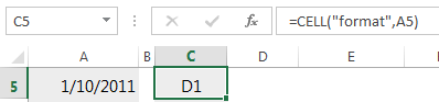
The result, D1, refers to the type of format applied to cell A5; ‘D’ for date and 1 for the type of date format, being dd/mm/yyyy.

It might not seem much use at first glance but I’ll show you some applications for it in a moment.

First some theory.…

CELL Function Syntax

The syntax for CELL is:

=CELL(info_type, [reference])

The info_type allows us to specify the type of information we want to return. We can choose from a long list:

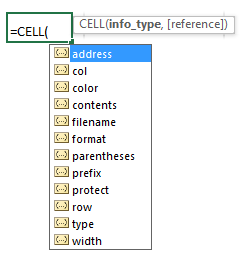
More on what each info_type means in a moment.

The reference is the cell we want to return information about. It’s an optional argument and if you omit it Excel will return the information for the last changed cell. Alternatively, if the reference is for a range of cells then you will get the information for the upper left cell in the range only.

CELL info_types

info_type	Returns
address	The address of the first cell in reference, as text. e.g $A$1
col	Column number of the cell in reference. e.g. a cell in column C would return 3
color	The value 1 if the cell is formatted in color for negative values; otherwise returns 0 (zero). Note: this is not the color of the text in the cell, it simply indicates if the format of the cell has special color formatting for negative values.
contents	The actual value of the cell; not a formula.
filename	Filename (including full path) of the file that contains reference, as text. Returns empty text ("") if the worksheet that contains reference has not yet been saved.
format	Text value corresponding to the number format of the cell. More on this below. Returns: "-" at the end of the text value if the cell is formatted in color for negative values. "()" at the end of the text value if the cell is formatted with parentheses for positive or all values.
parentheses	The value 1 if the cell is formatted with parentheses for positive or all values; otherwise returns 0.
prefix	Text value corresponding to the "label prefix" of the cell. Returns: a single quotation mark (') if the cell contains left-aligned text, a double quotation mark (") if the cell contains right-aligned text, a caret (^) if the cell contains centered text, a backslash (\) if the cell contains fill-aligned text, and empty text ("") if the cell contains anything else.
protect	The value 0 if the cell is not locked; otherwise returns 1 if the cell is locked.
row	Row number of the cell in reference. e.g. a cell in row 2 would return 2.
type	Text value corresponding to the type of data in the cell. Returns: "b" for blank if the cell is empty, "l" for label if the cell contains a text constant, "v" for value if the cell contains anything else.
width	Column width of the cell, rounded off to an integer. Each unit of column width is equal to the width of one character in the default font size.

 

CELL Function Examples

Ok, that’s enough theory, let’s look at some examples and then some practical uses for CELL.

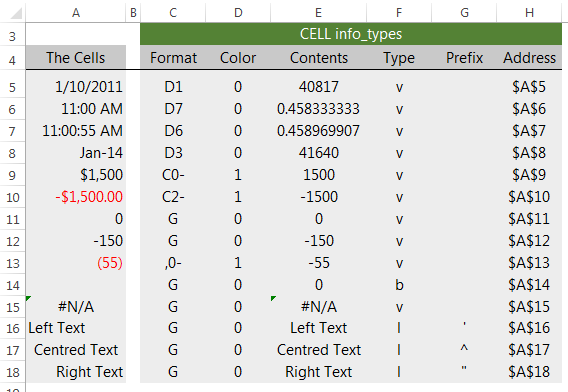
The table below shows the results for some of the different ‘info_types’ for the values in column A (that is, columns C through H contain CELL formulas which reference the values in column A):

Format Legend

The ‘Format’ info-type has a range of results. The table below explains what those results represent:

Result Returned	Actual Cell Format (as applied via the Format Cells Dialog Box)
"D1"	d/mmm/yy or dd/mmm/yy
"D2"	d/mmm or dd/mmm
"D3"	mmm/yy
"D4"	m/d/yy or m/d/yy h:mm or mm/dd/yy
"D5"	mm/dd
"D6"	h:mm:ss AM/PM
"D7"	h:mm AM/PM
"D8"	h:mm:ss
"D9"	h:mm
"G"	General
"F0"	0
",0"	#,##0
"F2"	0.00
",2"	#,##0.00
"C0"	$#,##0_);($#,##0)
"C0-"	$#,##0_);[Red]($#,##0)
"C2"	$#,##0.00_);($#,##0.00)
"C2-"	$#,##0.00_);[Red]($#,##0.00)
"P0"	0%
"P2"	0.00%
"S2"	0.00E+00
"G"	# ?/? or # ??/??

 

CELL Function Examples

Ok, now for some practical applications of CELL.

Ignore Cells with Specific Formatting

A while back Kyle wrote in with this question:

My cells contain one of the four things listed below  

1. random dates
2. the letter N
3. the letter I
4. N/A

I’m trying to write a formula that will give me a percentage of the cells that contain dates out of the total number of cells that I have selected. I would also like to exclude from the percentage listed above all cells containing N/A. How would l do that?

And Catalin, our in-house Excel Guru, replied with this solution using the CELL function:

Assuming that your range is in column A, starting from row 1, use this formula in cell B1:

=CELL(“format”,A1) and copy it down as needed.

Then you can count the results of the CELL formula and calculate the percentage with this formula:

=COUNTIF(B1:B8,"D*")/(COUNTA(A1:A8)-COUNTIF(A1:A8,"#N/A"))

Of course this formula relies on the cell format matching the data. It is possible to format a cell containing text as a date which would result in an error.

Return the File Path:

We can display the file path of the current workbook using this formula:

=CELL("filename")

Notice how we can omit the reference argument since the file name is not dependent on one cell.

The result is the file path, file name and sheet name:

D:\My Documents\Training\Blog\Excel CELL Function\[excel_cell_function.xlsx]Sheet1

This is handy for inserting the file name in my worksheet so that when I print the report the file path is visible. It helps you find the file months later!

You can put this in the header/footer too but it’s just as easy to use the CELL function in a cell somewhere.

File and Worksheet Name

The above =CELL("filename") formula can also be used in INDIRECT formulas to populate the worksheet name but you need to isolate just the worksheet name component from the whole file path first, which can be done with this formula:

="'"&MID(CELL("filename"),FIND("]",CELL("filename"))+1,256)&"'!"

Which will return:

'Sheet1'!

Note: with the single apostrophe at each end and an exclamation mark the worksheet name is ready for use in your formulas. The apostrophes are only required if your sheet name has a space in it, but it’s handy to put them in anyway because if you add a space to your sheet name later on your formulas won’t break.

More on using the MID function to extract text strings here.

Warning – Advanced Use of CELL

I learnt this tip from fellow Excel MVP, Jordan Goldmeier of OptionExplicitVBA.com

If you ever use the INDEX function to return a cell reference to a single cell you might want to verify that the formula is actually returning a cell reference as opposed to the value in the cell.

You can do so by wrapping the INDEX formula in a CELL function like so:

=CELL("address", INDEX(…MATCH()…))

The CELL function will return the address given by INDEX as opposed to the value that typically appears.

CELL Function Tips

• If you change the format of a cell you need to hit F9 to recalculate the formulas as it doesn’t automatically recalculate upon a formatting change.
• The info_type argument “Color” doesn’t refer to the color of the text or format of the text, it refers to whether the number format is such that it formats negative values in red, or any other color formatting applied through a custom number format.
• The CELL function isn’t a native Excel function, it’s actually provided for compatibility with other spreadsheet programs.

CELL Function Errors

#VALUE!: if your CELL formula returns the #VALUE! error it’s likely that the info_type argument supplied isn’t recognised by Excel.

#NAME?: The #NAME? error will appear if you don’t enter a valid ‘Reference’ argument or if you misspell the function name.