In its simplest form the Excel GETPIVOTDATA function enables you to extract values from a PivotTable report, but if you’re like me when you first tried to figure out how to use GETPIVOTDATA, you were less than pleased with the results. Understandably so, because in its default form it’s quite inflexible.
However, the benefit in using GETPIVOTDATA, as opposed to a regular cell reference, is huge in terms of reducing your ongoing workload in maintaining your reports.
Why? Well, PivotTable reports are typically being updated and, or changing shape as you add new data to the source and alter filters etc. If you link to a cell in a PivotTable with a regular cell reference and then the location of that data changes due to a refresh, or a filter or Slicer being applied, then all of a sudden your formula is returning the wrong information.
Not so with GETPIVOTDATA. If the location of your data moves then GETPIVOTDATA will still return it, assuming it’s still visible somewhere in your PivotTable report.
So, my objective with this tutorial is to convert you from a GETPIVOTDATA hater (harsh, but it rhymes ;-)) to a GETPIVOTDATA lover! I know, I’ve got my work cut out for me.
The trick with leveraging GETPIVOTDATA power is to replace the hard keyed arguments with nested formulas so the GETPIVOTDATA formula becomes dynamic. Sounds complicated but it’s not.
As an example, the ‘hard keyed’ arguments are those in red below:
=GETPIVOTDATA("Order Amount",$A$4,"Order Date",1,"Years",2009)
Note: if you're using Power Pivot PivotTables, please refer to the GETPIVOTDATA tutorial for Power Pivot as the references are slightly different.
Watch the Video

Download Workbook
Enter your email address below to download the sample workbook.
Turn GETPIVOTDATA On
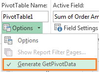
First, in order to have Excel generate the GETPIVOTDATA formulas you must have the preference turned on. If you’ve turned it off in frustration then you can turn it back on in the PivotTable Options tab of the Ribbon:
Excel GETPIVOTDATA Function Example
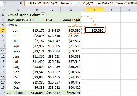
Let’s look at a simple scenario. You can see my PivotTable below. When I enter an equals sign in cell F7 and then click on cell D7 in the PivotTable, Excel automatically enters this formula:
=GETPIVOTDATA("Order Amount",$A$4,"Order Date",1,"Years",2009)
In English the GETPIVOTDATA formula reads, return the Order Amount for the Order Date (month) 1 (which is January) for the Year 2009.
Seems like a big formula for what would usually just be =D7, but remember there are big advantages to using GETPIVOTDATA.
Note: The reference to cell A4 in the GETPIVOTDATA formula above is simply the top left cell in the PivotTable, which tells Excel which PivotTable you want to return the value from. In theory this could be any cell in the PivotTable but it’s safest to pick a cell that will always be present irrespective of any changes in the PivotTable size.
Excel GETPIVOTDATA Function Relative References
The annoying thing with GETPIVOTDATA is that when you copy and paste the formula, for example down column F, the references aren’t relative. That is they don’t update like normal cell references to pick up the next cell in the range. So you end up with a column of identical values like these in column F:
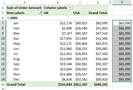
Right about now you’re annoyance levels are rising and if you’re working on a deadline you’re likely to revert to typing in the cell references because you haven’t got time to figure out how to STOP IT!
Making GETPIVOTDATA Formulas Dynamic
Let’s start by making the formula update so that it picks up each month when copied down the column. The trick here is knowing how PivotTables represent dates; while those months appear to be the month names Jan, Feb, Mar…, for the purpose of the Excel GETPIVOTDATA function, those months are actually numbers 1,2,3… through 12.
So we need to replace the month number argument in the GETPIVOTDATA formula with something that will count up automatically as we copy the formula down the column. For this we can use the ROW function.
ROW Function
The ROW function simply returns the row number of the reference. So, the formula ROW(A1) will return a 1, ROW(A2) will return a 2 and so on.
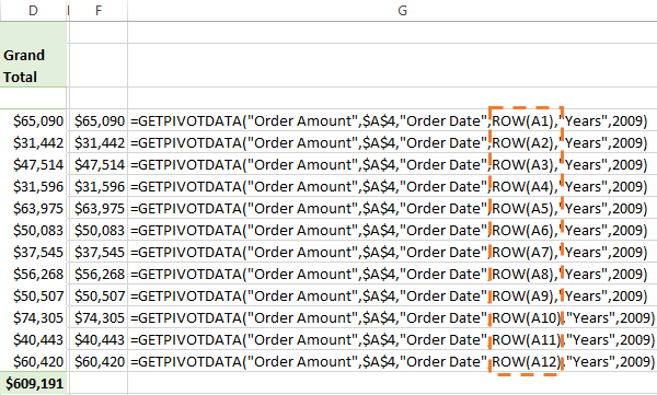
And we can put ROW in our formula in cell F7 like this:
=GETPIVOTDATA("Order Amount",$A$4,"Order Date",ROW(A1),"Years",2009)
Which evaluates to this:
=GETPIVOTDATA("Order Amount",$A$4,"Order Date",1,"Years",2009)
So now when you copy the formula in cell F7 down the column the relative reference to cell A1 in the ROW function dynamically counts up by 1. I’ve written out the formulas from column F in column G in the image below:
Now you might be thinking that's a fair bit of work just to make GETPIVOTDATA dynamic, when you could have just as easily entered =D7 and copied that down the column but remember, the benefits of GETPIVOTDATA mean a more robust formula able to withstand significant changes to your PivotTable without losing its place. The same can't be said for =D7. In this case you get what you pay for.
Tips:
- If you wanted to make the Year argument dynamic you could use ROW(A2009)….
- Or if your report had the years and months going across the columns you could use ROW’s cousin function, COLUMN instead:
The COLUMN function returns the column number of the cell reference, so COLUMN(A1) will return a 1, COLUMN(B1) will return a 2 and so on. - The ROW/COLUMN function can be used in other formulas to create a dynamic reference too.
Excel GETPIVOTDATA Formula with Data Validation
What if we wanted to get the grand total for each country and toggle between the two using a Data Validation List like this:
Our formula for the UK grand total would look like this:
=GETPIVOTDATA("Order Amount",$A$4,"Country","UK")
So all we need to do is link the country name argument to cell F3 which contains the Data Validation list like this:
=GETPIVOTDATA("Order Amount",$A$4,"Country",F3)
Now when you choose a different country from the data validation list the GETPIVOTDATA formula dynamically updates.
Easy peasy 🙂
Tip: Notice how there aren’t any month or year arguments in the formula above? That’s because we’re picking up the grand total.
Excel GETPIVOTDATA Function Tips
- I usually let Excel write my GETPIVOTDATA formulas by typing an = in the cell I want the value returned to, and then click on the cell in the PivotTable. This gives me a pre-written formula and all I need to do is edit it to make it dynamic. It’s a lot quicker than writing it out from scratch.
- You can make any of the arguments dynamic, not just the examples I’ve show you here.
- You can only use GETPIVOTDATA to pick up values that are visible in the PivotTable report. It can’t query the source data itself.
- You can use it to return values from Calculated Columns.
- Just like any other function, you can nest it in formulas or apply math/logic calculations on the result. e.g. you can add 10% to the value returned by =GETPIVOTDATA("Order Amount",$A$4,"Country",F3)*1.1
- If the value described by the arguments isn’t present in the PivotTable it will return the #REF! error.
Do you Love it now?
Please let me know if I've managed to convert you to a GETPIVOTDAT lover in the comments below. I'm dying to know!
If you use PivotTables then you must grow your love for GETPIVOTDATA. I don’t expect it to be love at first sight, but hopefully you now have some ideas on how you can leverage GETPIVOTDATA, and your fondness for it is starting to bloom 😉

Hi there, your video’s are fab. Thanks. Question – is it possible to make Field items dynamic? Figured out the items so that’s all good.
My pivot data headings are slightly different to the dashboard headings and so instead of Field1 being “Category” per the pivot data, I have a lookup table that references my dashboard headings to those of the pivotdata. I just can’t work out how to incorporate an x or vlookup into this part of the getpivotdata function.
GETPIVOTDATA(CONCATENATE(Lookup!$B$8),'[Pivot Input file.xlsx]Output’!$A$9,”Category”,Lookup!$F$6,”Solution/Service”,$C3,”Region original”,”RE”,”Fiscal Period”,VLOOKUP(Inp_RE_YTD!N$2,’Inp BSC’!$AG$16:$AI$27,3,0))
Thanks!
Hi Tam, yes you can use a lookup to return the field heading GETPIVOTDATA recognises. It looks like you’ve inserted the VLOOKUP where the item name is, not the field name.
It never occurred to me to use something like ROW(A2009) to sequence the years; what a great tip.
I never used the getpivotdata in any of my formulas before, I always used the cell address and ensured the table was set up in a way so it would not shift upon updates, but after this post, it looks like I will start.
I use a lot of time and date based pivot tables; summing time is always a challenge this process of using the getpivotdata may help.
So pleased you’re a GETPIVOTDATA convert, Rick 🙂 I’m sure you’ll be glad you used it going forward.
Is there a way to reference a whole column in a pivot table?
GETPIVOTDATA seems to be limited to a single cell value.
Such a dynamic column reference is needed when trying to apply conditional formatting to a pivot table, as visible values change when you try different filters.
Hi Luis, Yes, there is a specific technique for applying conditional formatting to PivotTables so that the formatting expands with the PivotTable. Mynda
What if I want to GetPivotData function to get a grand total that is generated by the pivot table? So For example, the pivot table is expense data organized with years in each column and the Grand total is the last column. How do I make a selection of cells (ex. M2:M10) from the grand total column?
Hi Dustin, simply type =GETPIVOTDATA( in a cell then click on the PivotTable cell containing the Grand Total and press ENTER. The formula will continue to track the Grand Total as the PivotTable expands or contracts.
=GETPIVOTDATA(“[Measures].[Visit Count]”,$B$8,”[Date Clinic Activity].[Clinic Month Name]”,”[Date Clinic Activity].[Clinic Month Name].&[7]”)
I want to drag the formula horizontally, withouth having to change [7] to [8], [9] etc
The field reads as July but in formula as [7]
Data is coming from a data warehouse so I can not alter field types.
Jul-19 format I get away with ‘&[“&MONTH(e$9)&”]” but above is obviously stored as a different date format
Is is working if instead of &[“&MONTH(e$9)&”]” you use &”[“&”July”&”]” ?
How can we use get pivot formula if we have converted pivot to calculate distinct count?
Depends on what you need. Can you give us a clue on what you need to do?
Wish I’d seen this a month ago. I’ve just created an energy report that uses a large amount of Pivot table data as a reference, and you described me exactly when I realized I couldn’t just drag my ‘=GetPivotData’ reference across and down the page so ended up having to use =D7, =D8 etc. Maybe I’ll go back and change it now because as you’ve just pointed out, if the pivot column ref changes my data will be wrong !! Excellent post, clear and easy to understand. Not sure I’m a GetPivotData Lover yet but we’re hoping to get to know each other a little better in the future.
🙂 better late than never, as they say. I’m sure your relationship with GETPIVOTDATA will blossom 😉
Good morning,
I like this option, but it’s not working for me.
I wanted to use it not with a date, but to refere it to a partnumber.
So I thought I have to replace “[Merge_AOP_BOM].[Material].&[M0171A974]” and I replaced it by ROW(B17)
But I get the #REF!
Can you tel me what I do wrong?
=GETPIVOTDATA(“[Measures].[Total Demand_PC]”,$B$15,”[Merge_AOP_BOM].[Material]”,”[Merge_AOP_BOM].[Material].&[M0171A974]”,”[Merge_AOP_BOM].[Source]”,”[Merge_AOP_BOM].[Source].&[AOP2019_OE(S)_20181127]”,”[Merge_AOP_BOM].[PLANT]”,”[Merge_AOP_BOM].[PLANT].&[03 Hodkovice]”,”[Merge_AOP_BOM].[UoM Basic Data]”,”[Merge_AOP_BOM].[UoM Basic Data].&[EA]”,”[Merge_AOP_BOM].[SAP_PLANT]”,”[Merge_AOP_BOM].[SAP_PLANT].&[HOM1]”)
=GETPIVOTDATA(“[Measures].[Total Demand_PC]”,$B$15,”[Merge_AOP_BOM].[Material]”,ROW(B17),”[Merge_AOP_BOM].[Source]”,”[Merge_AOP_BOM].[Source].&[AOP2019_OE(S)_20181127]”,”[Merge_AOP_BOM].[PLANT]”,”[Merge_AOP_BOM].[PLANT].&[03 Hodkovice]”,”[Merge_AOP_BOM].[UoM Basic Data]”,”[Merge_AOP_BOM].[UoM Basic Data].&[EA]”,”[Merge_AOP_BOM].[SAP_PLANT]”,”[Merge_AOP_BOM].[SAP_PLANT].&[HOM1]”)
Hi Johan,
Great to see you’re giving GETPIVOTDATA a chance 🙂
The ROW function is returning 17, so unless your part number is 17 you’re going to get an error. If you have part numbers in cells then you can reference those cells in place of the hard keyed values in the formula. I suggest you post your question on our Excel forum where you can upload a sample file or screenshots so we can help you further.
Mynda
Hello!
I’m trying to figure out how to set up a function where it sums the values when the Item Value contains part of a string. Example would be if the Row Values in Column A [Product] are “blue book”, “red book”, “yellow magazine”, and Column B is [Sum of Sales]. If i only wanted to capture Sum of Sales for the rows which contain “book”, how would I do it? I’ve tried this:
=GETPIVOTDATA(“Sum of Sales”, $A$1, “Product”,”*book*”)
but I got an #REF! error. I also tried to set up a cell with *book* and referenced the cell instead, but same error.
I know I can do this with the Field name, which would be:
=GETPIVOTDATA(“”&”Sales”, $A$1, “Product”, “blue book”)
but concatenating the empty string value didn’t work for the Item Value.
Thanks for any assistance you can provide (even if it’s to confirm it can’t be done)!
Hi Stacey,
You can’t use wildcards with GETPIVOTDATA. It’s looking for a specific field name, so if you have multiple fields with ‘book’ in them, how will it know which one to return?
Why don’t you filter the PivotTable to only show items that contain ‘book’. Then you can use GETPIVOTDATA to return the total of the filtered PivotTable.
Mynda
In the above last example (Excel GETPIVOTDATA Formula with Data Validation), how would I get the monthly average for any of the countries?
Hi Mariano,
That depends on the way you set the pivot table. For example, it does not matter if you use SUM , AVERAGE, MIN, MAX or COUNT as the aggregation type of that field, GETPIVOTDATA will return that result.
All you have to do is to set the aggregation for that field to AVERAGE.
Catalin
GETPIVOTDATA formula is great, but it will not work if the pivot table that provides the data is from a separate, closed workbook. So, if that workbook containing the pivot table is closed, you will get #REF errors. Is there a workaround to this? Will another formula work even if the source workbook is closed, like a SUMIFS perhaps?
Hi Gene,
I’d build the PivotTables in the file you want the GETPIVOTDATA formulas in. You can leave the source data in the other file and simply use it as the source for your PivotTable. This is the safest approach.
Mynda
In theory, GETPIVOTDATA is the bomb.com! I notice that when I update my source document, though, the system gives me a message that there is not enough memory to complete the update, and all I am doing is adding 3 rows with 67 columns. So there has to be an issue with my formulae:
Any suggestions for what glaring error I’ve included? =GETPIVOTDATA(“Referral Number”,RefStart!$A$3,”Ref Start”,COLUMN(E7),”Years”,2018)
Hi Sandra,
Are you sure it’s GETPIVOTDATA that’s the problem? Have you tried removing the formulas, adding new data and refreshing to check it’s not just the PivotTables that are the issue?
Mynda
How can we pass the multiple values from filter to the get pivot data function
Hi Venkat,
The GETPIVOTDATA function just returns data from a PivotTable. It will automatically pick up any filters, whether they’re single or multiple items and return the correct value. You don’t have to specify them in the formula. I would just build a PivotTable and link to the value you want to return. This will give you the formula arguments you need and the PivotTable will do the rest.
Mynda
Hello Mynda I am trying to use a validation list of 4 geographies which works great but what if I want to grab the total of all 4 geos.
=IFERROR(GETPIVOTDATA(“Sum of AAF AMT”,’PIVOT MES’!$A$3,”Mês”,AT$4,”FY”,$AR$4,”geo nm”,$AS$1),0)
is what I’m using with AS1 being the location of the validation list. If I want to grab the Grand Total then my validation list is “total geographies” but how do I make the Getpivot formula grab the grand total instead of the Geo Name total? I don’t want to add an if/then as I have about 20 rows and 12 months across that would all need that logic. Thanks in advance.
Hi David,
There are a few approaches to this, but without seeing how complex your 20 rows x 12 columns of data is, it’s difficult to say. My first thought is to just add an IF e.g.
=IFERROR(IF(data validation selection = “Total Geographies”, GETPIVOTDATA(reference the Grand Total), GETPIVOTDATA(“Sum of AAF AMT”,’PIVOT MES’!$A$3,”Mês”,AT$4,”FY”,$AR$4,”geo nm”,$AS$1),0)
If that approach is too much hassle, then please post your sample Excel file and question on our Excel forum where we can help you further.
Mynda
Thanks, I’ll give that a go.
Hi Mynda
First and foremost, nice article! As usual 🙂
The bit I might challenge is “knowing how PivotTables represent dates”.
If you test a month name within the table with ISTEXT or ISNUMBER it comes up as text.
If you write {“Jan”;”Feb”;”Mar”} into a helper range (or a named array constant) and reference that you get the correct results. It would appear that it is a trick of GETPIVOTDATA that permits you to use a numerical index instead of a text string.
I suspect that using ROW to generate a sequence of numbers, though an interesting topic in its own right, is something of a digression in this context. A helper range would do.
Something else that might be of interest is how to use a pivot table to generate such a list of unique items in the first place.
Thanks, Peter. Good points 🙂
Mynda
Hello, Mynda,
It is a very good information. I highly appreciated it. However, how do I bring this dynamic behavior onto Pivot Chart?
My Pivot Chart value should dynamically change as I change slicer. Do you have an example to share? I will feel much obliged. Thank You.
Hi Sam,
Your Pivot Chart will respond to changes in the Slicer just the same as the PivotTable does since they are linked. Have you tried it?
If it’s not working please post your question and sample file on our Excel forum so we can take a look at what might be causing the problem.
Mynda
Great piece! Thanks a lot!
You say this:
If the value described by the arguments isn’t present in the PivotTable it will return the #REF! error.
I am applying a slicer (filter) that causes the #REF! for me b/c, as you say, the value isn’t present in my Pivot Table. Do you know of any way to insert logic that goes as follows?:
If value doesn’t exist, return zero
Appreciate any thoughts.
Hi Zach,
Sure, you can use IFERROR to hide the error e.g.:
You can learn more about IFERROR here.
Mynda
hi Mynda, I try to do example by changing the text arguments dynamic but it shows #Ref error. example, the bat man is show in row A1.
GETPIVOTDATA(“Sum of Viewers”,$A$3,”Program”,”Bat Man”)
Please advise.
Hi Estella,
It looks correct so there must be more to it and I will only be able to tell if you send me your file, or you can raise your question on our Excel Forum.
Mynda
Thank You so much Mynda that was so helpful!
However I am trying to automate the formula on my worksheet so that it enters t\data from my PivotTable automatically without me typing( =) and selecting the preferred cell from my PivotTable in every cell in my new worksheet.How do i go past that .And when i copy the formula , there are lot of fields which need to be changed but i dint know how.
Kind Regards….
cheers
Hi Nathan,
See the “Making GETPIVOTDATA Dynamic” in this article, you will find there a simple method to change static parameters to dynamic.
If you get stuck, you can always open a new ticket on our help desk, with a sample file.
Cheers,
Catalin
I’ve had enough of skirting round GPD, and before a long weekend, I want to get to grips with it, but when I try substituting the item arguments with the row and column functions I get a #REF! error.
Original formula was :
=GETPIVOTDATA(“Total Cost”,$A$1,”CSU DRUG”,”ABACAVIR”,”CSU BUDGET CATEGORY”,”AIDS/HIV ANTIRETROVIRALS”)
I tried changing it to :
=GETPIVOTDATA(“Total Cost”,$A$1,”CSU DRUG”,ROW(A1),”CSU BUDGET CATEGORY”,”AIDS/HIV ANTIRETROVIRALS”)
Does it make any difference if I have more than one field in the row label box? (I’m currently using Excel 2007.)
I’m hoping this’ll prove to be like gold dust, like manipulating the SERIES function.
(I love the name “Sippy Downs”, it sounds so . . . . . Australian!)
Hi Tim,
No it won’t make any difference if you have nested row labels.
I think the problem is that you replaced “AVACAVIR” with ROW(A1). ROW(A1) returns a number, but I suspect the field you’re trying to find contains text more along the lines of “AVACAVIR”. Why are you using ROW(A1) and not a cell reference?
Mynda
P.S. Sippy Downs sounds like rolling hills of green. It probably was once, but not anymore!
Hello Mynda,
Shows I probably don’t quite understand, but I thought by changing ABACAVIR (the first item in my list of drugs) to Row(A1), Row(A1) would return 1 and so GPD would pick up the total cost for the first item (ABACAVIR). Seemingly not.
Don’t worry about replying straightaway. This can always wait till next week. Must be night time in Queensland.
Kind regards,
TimC
Hi Tim,
It’s hard to give you an example that will make sense because I can’t see your file, but the cell reference must be pointing to a cell which contains the name of the item you want the value returned for. e.g. if cell F1 contained the text “ABACAVIR” then you could write your formula like this:
=GETPIVOTDATA(“Total Cost”,$A$1,”CSU DRUG”,F1,”CSU BUDGET CATEGORY”,”AIDS/HIV ANTIRETROVIRALS”)
i.e. you have to give Excel the name of your row label, not the number.
Hope that makes sense. If not please send me your file via the Help Desk and I can be more specific with my examples.
Mynda
P.S. it’s gone 9PM 🙂
Hi Mynda,
I have loved GPD for a long-long time so I wanted to use also with PowerPivotTables. I have just realized that the syntax is different though so I cannot easily swap a field name to a cell reference.
Is there a way this could work? Can you please share a correct syntax to change let’s say “[Master].[Segment].&[ABC]” to the value in cell B1? Thanks in advance!
Hi Rita,
Yes, I cover this in the Power Pivot course that you’re a member of. See session 7.10.
Kind regards,
Mynda
Hi Mynda,
I have similar problem.
I’m currently using Excel 2016, but it seems that Power Pivot is not available?
I have tried Options> Add-ins > COM Add-ins, but it s not there.
Would you please advise how can I do about this?
Hi Emi,
Unfortunately Power Pivot is not available in all versions of Excel. You need either Excel 2016 Office Professional Plus, Office 2016 Professional, Office 365 ProPlus, or in the standalone edition of Excel 2016.
If it’s not in your COM add-ins it suggests you don’t have a compatible version of Excel.
Mynda
@Rebecca
Hi Rebecca
the Excel GetPivotData function can seem like quite a handful when you first encounter it, but it is possible to parameterise all of the inputs it requires, by placing the values in cells, and then referring to those cells in a “universal” GetPivotData formula.
The first reference, which is the name of the Data field required, can be entered into a cell as text e.g. Order Amount, but when passing this as a parameter you have to Append a double quote, so if the text was in cell C1, you would have to enter into the formula C$1&””
The second reference which is the Sheet and cell reference of the top left cell of the Pivot Table, can again be entered into a cell as text e.g. Sheet2!$B$4, but when entering into the formula you need to wrap it in an Indirect() function, so if the text was in cell C2 of your sheet, it would be INDIRECT($C$2).
so the whole formula would look something like
=GETPIVOTDATA(C$1$””, INDIRECT($C$2),$C$3,$B12,$C$4,C$10)
where C3 held the name of your Row field
B12 held the item from that field that you wanted
C4 held the name of your Column Field
C10 held the item from the column field required
Hopefully, if you study the above alongside the article that I mention, you might be able to work out what you need to do.
As Mynda says, you should wrap the whole of the formula, as above, inside an IFERROR() wrapper
=IFERROR(GETPIVOTDATA(C$1$””, INDIRECT($C$2),$C$3,$B12,$C$4,C$10)
,””)
Mynda, great tutorial as always.
Thanks Roger – the last bit I was trying to rectify was answered by your ‘append double quote to the cell reference’ comment. That’s fixed my whole issue 🙂
Hi Mynda, your tutorials are always fantastic. However I’m still struggling to figure out if this can help me with my issue, or how to use it properly. I basically created a replicate table (in a 2nd worksheet) to copy data from a pivot table because I wanted to manipulate it in various ways, eg adding extra columns, splitting text using a power query etc – and I couldn’t do that within the pivot table. HOWEVER it all fell apart (of course) when I decided I wanted to add an extra field to the pivot table and the changes to cell references destroyed all my formulae.
I think getpivotdata should be able to help, but cannot get it to work because Excel is not automatically generating a ‘getpivotdata’ formula (despite having it turned on in options) and I can’t figure out what to enter for the data_field, fields and items. The pivot table contains row labels like Profit Center, Project and Program and column labels like Expenditures and Revenues. I need to replicate all of these.
I tried using:
Data_field = the cell in the pivot table that holds the column heading I want to return (eg. ‘Pivot’!A14 = “Profit Center”)
Pivot_table = the top left hand cell of the pivot table (‘Pivot’!A14)
But I can’t work out what the Fields and Items should be. Whatever I try, I get an error. It’s driving me crazy!
Hi Rebecca,
Great to hear you’re giving GETPIVOTDATA a go.
GETPIVOTDATA only works on the values area of the PivotTable. The row/column headings are not something GETPIVOTDATA can reference. For those cells you can only use regular cell references or formulas.
You should be able to re-create your PivotTable with a combination of regular formulas and GETPIVOTDATA if you build in error handling with the IFERROR function.
If you’d like me to look at the workbook or a sanitised sample of it, you can send it to me via the Help Desk.
Kind regards,
Mynda
Thanks, Mynda – a great training tip on the GETPIVOTDATA Function. Easy to follow and works great.
RL
Thanks, Roger. Glad you liked it.
Mynda
Another fabulous article.
How would GETPIVOTDATA handle the same problem but instead of a date field, the row had text? For instance, regions, names, or products…. I found myself typing the text in every row of the GETPIVOTDATA formula – quite a nuisance for a lazy excel user.
Happy birthday to your big and little boy – the world revolves around 6 year olds.
Gráinne
Hi Gráinne,
Glad you liked it 🙂
You could put the names/regions/products in a column/row adjacent to your formula and then reference those cells. If they’re names you use all the time then you can set them up in a Custom List so you can use autofill to quickly populate the cells.
Thanks for the birthday wishes. I’ll pass them on 🙂
Mynda
Hi Mynda,
Nice article again!!
I would consider myself an “avoider” to an “accepter” and finally a “promoter” of GPD.
One side topic:
I think the use of ROW(A1) could be dangerous. I always encounter users who have a great tendency of “destroying” spreadsheet… 😛 Think about if a user delete the entire row 1 or column A…
Normally, I use GPD mainly for “re-layout” a PT (it’s strange to say that as PT is supposed to be “re-layout” easily, but I think you understand what I mean), I would rather put the variables into visible cells next to the GDP formula, and referencing to the cells carrying the variables.
or
ROWS($1:1) as an alternative
Cheers,
Cheers, MF.
I usually use ROW($1:1) too, but I thought the concept was easier to understand with A1, so opted for that. I also like the inputting variables into visible cells adjacent to the formula. Good ideas. Thanks for sharing.
Mynda
Below is a comment emailed to me from Bryon Smedley that I just had to share on the blog:
I’m not completely against GPD, but I’m not convinced by Byron’s argument for using it, viz:
“…it’s far easier to create a quick-n-dirty pivot table, and then point to key cells in the table and extract the gems with GETPIVOTDATA then it would be to create relatively more complex SUMIFS, AVERAGEIFS, COUNTIFS, or SUMPRODUCTs…”
I see no point in adding an intermediate structural element to a workbook when SUMIFS, AVERAGEIFS, COUNTIFS, SUMPRODUCT, etc.:
1) can return the desired result directly and far more transparently than GPD,
2) can utilise structured and/or external referencing in the same way as GPD, and
3) which are less easily corrupted (i.e. by design, PivotTables are a dynamic analysis tool, so any re-arrangement of the fields reported therein can result in the GPD function returning an error.)
Thanks for sharing your view, Col.
I think PivotTables tend to be more efficient when working with large volumes of data than the ‘IFS functions. I reckon I could write a PivotTable with a series of ‘IFS equivalent values in a fraction of the time it would take to write those same ‘IFS formulas with a few criteria. I’m not sure I agree that a PivotTable or GPD formula are any less transparent than ‘IFS formulas, although I do agree that Structured References make formulas much easier to read and write.
In terms of GPD returning an error, it will only return an error if the data is no longer anywhere in the PivotTable. You can move columns to rows and vice versa, apply filters etc. and GPD will still find the value.
Don’t get me wrong. I love the ‘IFS functions too and they have their place, particularly if you just want to return one value, but I think PivotTables and GPD are more robust in large data models.
Cheers,
Mynda
Mynda,
This post just forced me to re-look at GPD function afresh – I had actually given up on it. After reading through your post i came off feeling like you have loosened some knot to were too tight for me to untie.
i have been meaning to automate some management reports from data that come from SAP.
I believe once i get my head round this GPD function, then I will be able to complete that project successfully.
cheers for such a great post
Philip
You’re welcome, Philip. Glad I could reignite your GPD fire!
Mynda
Don’t love it yet, but a great post! I never really wanted to do much with GetPivotData because I did not understand it very well and was frustrated with some of the limitations that are mentioned. This opens up a whole new world and I am now much more willing to give it a try when the need for something like this arises – at which time, I am sure I will be glad for this post. Thanks, Mynda!
Mynda kept it appropriately simple, but for some additional thoughts, I could easily see putting a column for the months to the left of the GetPivotData column that Mynda shows. The GetPivotData column would reference the new column. This could make it even more dynamic (or easily updated) than the great example of using the row function. With this type of capability, I could easily see moving the GetPivotData to a whole different worksheet and building a regular chart off of the table we just built with the GetPivotData. This would allow us to get past some of the limitations of pivot charts. And as Mynda alluded to, we could wrap the GetPivotData formula in an “iferror” function to appropriately take care of the months (or other situations) where they may not be any data.
Hi Paul,
I’m glad GPD is growing on you 🙂
Great ideas for further/alternate automation. Thanks for sharing.
Mynda
Thanks Mynda
This was a very helpful tutorial,
I’ve encountered the “non-dynamic” issue with the GetPivotData function and resorted to the = CellAddress workaround.
This is a much better fix, concisely explained, and simply demonstrated ( as usual) .
Thank you
You’re welcome, Rachael. It’s fantastic to know you’re warning to GPD 🙂
Sweet. I’m only just starting to break the ice on Pivot Tables and this helps. Well done example. Thank you for posting and thank you for using G+.
Thanks, Tom 🙂 Keep going with the PivotTables as they’re a great Excel skill to have.
Thanks, Mynda. Always great to keep learning more in Excel!
Cheers, Mike.
Awesome post. Really valuable tip. Didn’t know that trick. Thanks for posting it.
Thanks, Jef. Great to know you found it useful.
Cheers,
Mynda
I’m definitely going to try to fall in love with GPD. People are always wanting to manipulate the PT to see data their way. I have to put a note at the top of the page to state that changing the PT will cause the formulas to fail. I then create a copy of the PT to allow them to manipulate as they please. This increases the size of the workbook and takes longer to open and refresh.
By using GPD, they can insert all the columns they wish and the formulas will still work. Thanks for the little shove!
🙂 you’re welcome, Mike. The warning might still be required but hopefully the breakages will be less.
Hi Mynda,
Is it because I am referencing a PowerPivot table or because I have the “Use table names in formulas” option ticked that I am getting the following syntax?
=GETPIVOTDATA(“[Measures].[List Price]”,$E$2,”[Products].[Business Line]”,”[Products].[Business Line].&[01 Crisps]”,”[Products].[Product Group]”,”[Products].[Product Group].&[12 Pringles]”,”[Products].[Product SubGroup]”,”[Products].[Product SubGroup].&[0001 Pringles Small x 12]”,”[Products].[Product]”,”[Products].[Product].&[PR029 Pringles S&V 40G]”)
Is the usage of formulas as suggested restricted to elements that are represented as Month Nos, Day Nos etc?
Hi Ted,
It’s because the PivotTable you are referencing is a Power Pivot PivotTable. i.e. you have created a Power Pivot model and then created a PivotTable from that model.
Whenever you see ‘measures’ you know you’re referencing a Power Pivot PivotTable.
You can still apply the concepts I mention in my tutorial above to a Power Pivot PivotTable, but you have to allow for a slightly different formula structure that uses the Structured Reference style of referencing, much like Excel Tables.
The formula you mention doesn’t have any date elements like in my example but, you could use nested formulas to toggle between different product SubGroups etc.
Phew…. Maybe my Power Pivot course would be of interest to you 🙂
Please let me know if you have any other questions.
Kind regards,
Mynda
Hi Mynda
Excellent article, as always
@Ted
I may be wrong, but as far as I can see, Ted has no reference set as to the location of the PT. GPD needs a sheet and cell reference to the PT (and as you said Mynda, use the top left cell by choice).
Without that information, GPD cannot determine the PT name, hence it will always error out.
@General
All of my financial reports access a PT for their data.
The Months or Quarters appear in a given row, in an identical format to the PT Columns values.
Going down the left hand column of my report are the Rows values that I wish to pick up from the PT.
Using this structure, I am always referencing cell values, and, making the Row column absolute, and the Column row absolute my single formula can be copied down or across to generate the report.
e.g.
=IFERROR(
GETPIVOTDATA(“Amount”, ‘ Data field
PT_Trad!$B$5, ‘ PT location
“Analysis”,$B7, ‘ Row field (absolute column ref)
“Inv month”,C$5), ‘ Column field (absolute Row ref)
“”)
And whilst you point out that GPD is an extremely efficient function that will find the data from the PT even as the PT changes, it might be noted that this only works if the PT is expanding in length or width, or if the order of the rows or columns alters.
If the PT structure alters e.g. more Row items or Column items are added, then GPD may error. It all depends upon where the new fields are added.
In the example above, Analysis is the first (and only ) Row field and if I were to add another Row field, e.g. Trader and place this below Analysis then GPD will work, but if I place Trader before Analysis then it will fail (quite rightly).
Similarly with the Column fields, bringing in any other field as well as Inv Month will cause GPD to fail, other than bringing in Year. Whether this is by design, or a “quirk” I do not know, but it seems to be the case.
If you wanted to make your report even more flexible, allowing you to switch things round so Months go down the report page and Analysis across the columns, you can enter cell References in place of the fixed titles for the PT fields
For example, if you entered Analysis in cell C1 and Inv Month in D1, then the formula could be
=IFERROR(
GETPIVOTDATA(“Amount”,PT_Trad!$B$5,$C$1,$B7,$D$1,C$5),
“”)
Now, if you entered your Month headings in cells B7 downward and your Analysis headings in C5 and across, then by switching the contents of C1 and D1 your report would alter without changing your formulae.
Equally, if you wanted to change your report to a Cash Report, then in your PT you could put Pay Month as the Column filed in place of Inv Month and then just type type Pay Month in cell D1 in place of Inv Month.
The only part of the GPD formula you don’t seem to be able to set as a cell parameter, is the very first item “Amount”, or the field that you have chosen for your Data area of the PT.
Sorry to have gone on for so long, but your article has appeared just at the time I am completing an article myself on GPD, and taking a slightly different slant on it. I will let you know when the article is published.
Best wishes
Roger
Cheers, Roger. Thanks for sharing your PivotTable expertise with us.
I look forward to your article.
Mynda
The potential problem identified by Roger in @General is precisely why I think using the native functions such as SUMIFS, etc. to directly return the values required is a better/safer option and which is just as quick overall (i.e. after building PT and then referencing it with GPD formulae). I can see little value in incorporating the intermediate structure of a Pivot Table (that is easily inadvertently changed) to create reports or return values that are relatively static in nature (e.g. financial statements). All that is doing is creating another avenue for error.
But who knows, one day I may yet come to love GPD, though at the moment I think she’s more trouble than she’s worth, and there’s far more attractive, interesting, and trustworthy options to pursue!
Avagooweekend
Col
@Col
Forgive me if I disagree with you.
I was not saying it was a problem, merely pointing out that GPD formula WILL need to be adjusted if you DO change the PT layout.
For all of my client’s reports, they never ever see the sheets with the PT’s as these are Very Well Hidden, and the workbook password protected so they can never get at the PT’s to make any changes.
In such a scenario, there is never any risk of GPD getting it wrong.
The PT is FAR more efficient at doing all of the “heavy lifting” compared with having to write a whole heap of SUMIFS, and in fact my final GPD formula that I posted is one I can just copy and paste to any report that I like, and just adjust the parameters held in C1 and D1 and I’m “good to go”.
A quick Search and Replace “Amount” with the name of the Data field and my new report is set up.
So, whilst I am supporting GPD here, and trying to show how, in addition to all of Mynda’s good advice, you can use it quickly and easily, I do have a very good alternative to GPD – but you will have to wait until I publish my article to see that.
I do agree though, that SUMIFS and it’s relations, are extremely fast and efficient functions and have the intelligence to deal with only the used range of a spreadsheet, even if you throw whole column references at them. Along with INDEX and MATCH, they are the “bid daddies” of the Excel functions in terms of speed and efficiency.
But, whatever method is used to extract data from a PT, using a PT to do all the work will always be my favoured method, as I think that PT’s are the real “hidden gem” within Excel and don’t even get me started on Power Pivot!!!!
Likewise, I wish you a great weekend.
Roger
Roger Govier – Excel MVP (so probably very biased about PT’s!!)
Ok. You talked me into trying GPD again. I am constantly having to repair broken reports due to updates. I will let you know how it goes.
Thanks for all the good info.
Yay! Good luck with it. I’m sure once you tame it you’ll love it.
Mynda
Hi Mynda
I think I need some further schmoozing from GETPIVOTDATA before I’m in love with her – she’s high maintenance!
When you say “…. while those months appear to be the month names Jan, Feb, Mar…, for the purpose of the GETPIVOTDATA function, those months are actually numbers 1,2,3… through 12.” is that because the underlying values are entered this way in your example, or is the PivotTable assigning index numbers (1-12) to the items in that PT field?
Thanks
😀 too funny. I always pictured GETPIVOTDATA as a man but it would make more sense to think of her as a ‘she’, given the high maintenance aspect!
The PivotTable changes the underlying date serial numbers found in the source data to the index numbers 1-12.
Cheers,
Mynda
Mynda, thanks. I routinely have to copy/paste special (values and number formats only) outside of the pivot to calculate cumulative totals by month into incremental amounts … this tip will definitely save time, once I’m familiar with using it a couple times. I only wish (since these amounts are normally in columns and one row) I could copy/paste the formula to the appropriate “next” row (e.g. three rows down) and have it automatically pick up the “New” row, but if that works, I didn’t figure it out this morning.
Either way, thanks again,
Keith
Hi Keith,
I didn’t understand what you meant by copy/paste the formula to the appropriate ‘next’ row. Perhaps you could send me an example via the Help Desk and I can help you find a way to automate it.
Cheers,
Mynda
Do you mean “Running Total” which can be actually done within the PT?