Conditional Formatting PivotTables

Conditional Formatting in PivotTables has its ups and downs. Unfortunately I find them mostly ‘downs’ but let’s not dwell on the negative as the few ‘ups’ might still make it worthwhile depending on your needs.

The Upside of Conditional Formatting PivotTables

When you apply Conditional Formatting to the Values area of your PivotTable the formatting will automatically expand/contract as you add new data or make changes to the filters, rows or columns.

In other words, the Values area becomes a dynamic range for the Conditional Format without you having to do any extra work. Nice....and just as it should be.

Here’s a little diagram so you know what I mean by ‘the values area’ etc.:

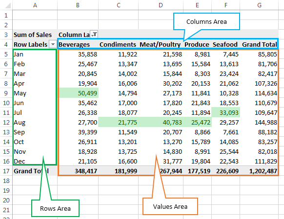
In the above PivotTable I have applied Conditional Formatting to highlight the top month for each column (except the Grand Total… in some instances that’s a downside since you might want the top month overall highlighted too).

Here’s a step by step how to:

1. Select any cell in the values area of your PivotTable

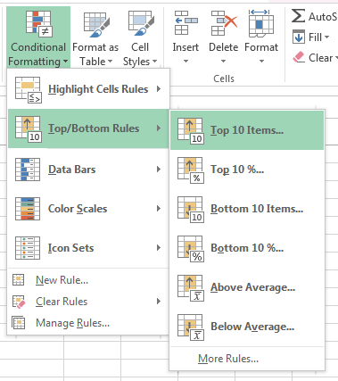
2. On the Home tab of the Ribbon select Conditional Formatting > Top/Bottom Rules > Top 10 Items:

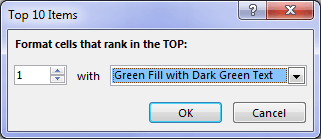
3. Set the value to 1 and choose your format:

4. You will now have an icon beside the cell that you have applied the formatting to. Click on it and select ‘All cells showing “Sum of Sales “ values for “Month” and “Category”:

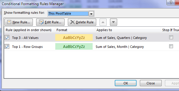
5. Then click on the Conditional Formatting button on the Home tab of the Ribbon and select Manage Rules. This will open the Rules Manager dialog box:

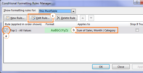
Notes on the image above:

a) Notice how the rule has a PivotTable icon at the far left. This is an indicator to let you know that this rule is applied to a PivotTable. If you’re familiar with Conditional Formatting you’ll know that rules applied to regular cells don’t have this icon.

b) The other thing to note is the ‘Applies to’ is a list of the PivotTable fields as opposed to a range of cells. When you see this you know that the range will dynamically update with any changes you make to the PivotTable.

6. Ok, moving on, click on the rule and then click the ‘Edit Rule’ button (labelled 'c' in the image above) which opens the dialog box below:

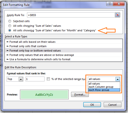
Tip: here you can also change the ‘Apply Rule to…’ we did back in step 4.

7. Click on the down arrow beside ‘all values’ and choose ‘each Row group’ > click OK > click OK again.

This will result in the top sales for each column (except the Grand Total) of your PivotTable being highlighted like so:

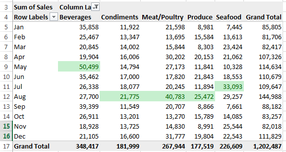
Now when you change the filters, add new data, or move the column/row fields around, the Conditional Formatting follows.

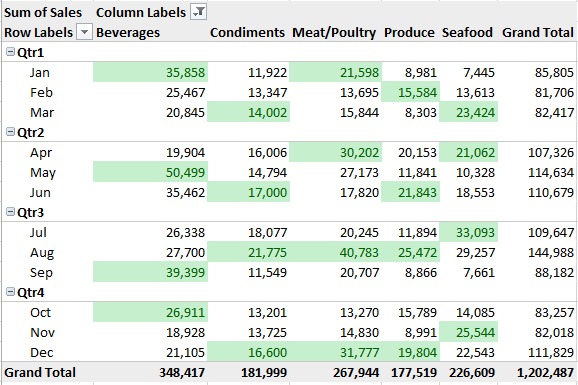
For example, changing the PivotTable Date Grouping to include Quarters results in the Top 1 result for each column per quarter being highlighted, without me changing the Conditional Formatting rules at all:

Why stop there? Actually you should stop but this is an example of what you can do, not what you should do so I’m going to make it a bit gaudier and apply formatting to the top 3 quarters next:

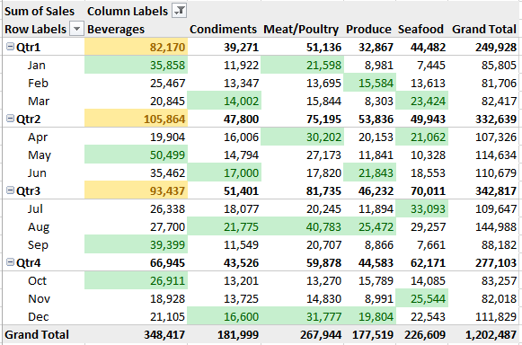
Now I have 2 rules in my CF manager; one for the top 3 quarters and one for the top 1 result for each column every quarter:

Want More?

Ok, I’ll give you more, but be warned the overuse of formatting might burn your audience’s retinas so proceed with caution.

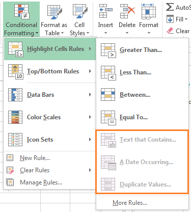
You can actually use any of the built in Conditional Formatting rules covered here, except these ones you can see greyed out in the menu below:

The Down Side of Conditional Formatting PivotTables

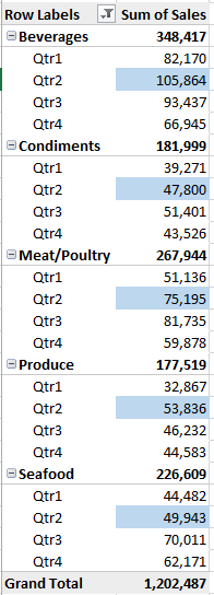
What say I want to highlight the ‘Sum of Sales’ amount for all instances of Qtr2 in the Row Labels, as I have done below:

My rule for the above formatting looks like this =$A3=”Qtr2” as you can see below in the CF Rules Manager:

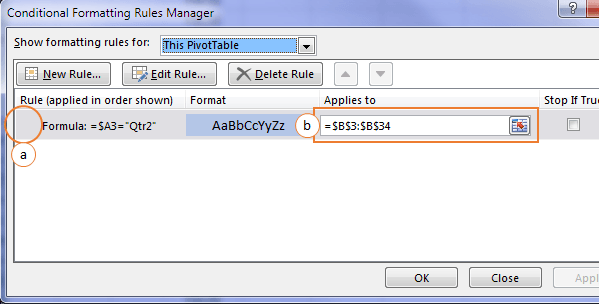
a) Notice the absence of the PivotTable icon in the far left. This is the first indication that Excel doesn’t recognise this as being applied to a PivotTable and,

b) The ‘Applies to’ range doesn’t have the PivotTable fields listed. Instead it is an absolute cell range. So as you change the PivotTable layout or add new data, this range is likely to become fragmented and you may get inconsistent results.

The Bottom Line

If you want to use any logic rules that rely on the Row or Column labels be prepared to update the ‘Applies to’ range each time you refresh the PivotTable or make any changes that alter the size.

This is a pretty big downside since some of the most useful Conditional Formats are applied based on the TRUE/FALSE outcome of formulas. Sure the built in rules are ok, but I mostly tend to use formulas to define my formats.

Side note: You might be thinking that you can just set up a dynamic named range to use in your ‘Applies to’ criteria for the Conditional Format however, as soon as you enter a dynamic named range in the ‘Applies to’ field and press ok, Excel converts the range to cell references rendering it non-dynamic (is that a word?). Ugh! Frustrating, yes, and a pretty big downside.

The only way I know of to get around this is with VBA, but it’s complicated and I’ve run out of time to cover it here. I’ll try to persuade Phil to address this in one of his future VBA posts.