Imagine examining hundreds of rows of raw data in Excel in an attempt to find a pattern or trend. You’d go mad!
Thankfully one of the tools we can use to make this task simpler is Conditional Formatting.
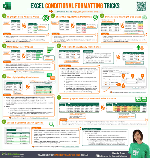
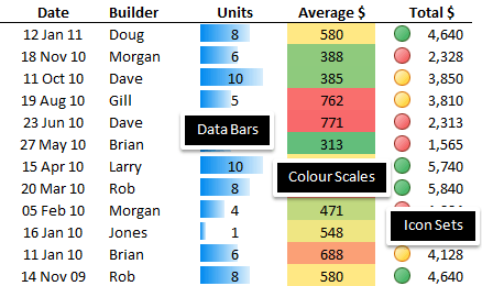
Excel includes many default Conditional Formats, including colour scales, icon sets and data bars to name a few. More on these below.
Table of Contents
Get the Practice File and Cheat Sheet
Enter your email address below to download the free files.

When to Use Excel’s Conditional Formatting:
- If you want to be informed in real time
- Answer questions visually
- Analyse data: find exceptions, find relationships, find trends, etc
- Enhance data presentations
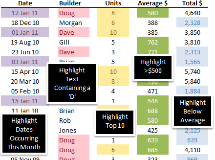
You can choose from inbuilt rules like:
- Top 10 or Bottom 10 using percentages, average or item
- Greater than, less than or equal to
- Text that contains a specific word or phrase
- A date occurring
- And even identify duplicate values
Or you can insert a formula and create a custom conditional format. More on that later.
Colour coding can be simple like font colour, font style and cell fill, or more elaborate with icons, colour scales or data bars.
Examples
How to Apply Conditional Formatting:
- Select the range of cells you want formatted.
- From the Home tab go to the Styles group and select Conditional Formatting.
- The menu will appear with your formatting options.
- When you choose one of the options a cascading menu will appear.
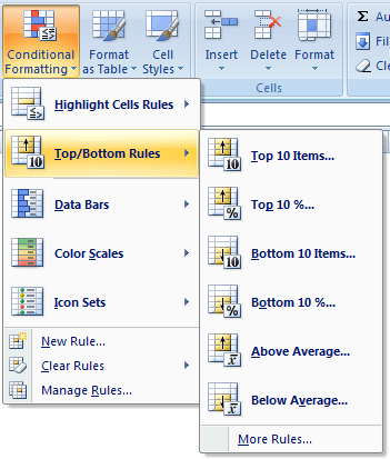
- Depending on which option you choose you will be prompted to make more selections.
- Note: You can specify a custom format or use one of the defaul formats. You can choose to format the cell fill, font style, colour, size, bold, italic, underline and more.
Remove Rules:
- Click the Conditional Formatting command.
- Select Clear Rules. A cascading menu appears.
- Choose to clear rules from the entire worksheet or the selected cells.
Manage Rules:
- Click the Conditional Formatting command on the ribbon.
- Select Manage Rules from the menu. The Rules Manager dialog box will appear as below.
- You can change the list of rules displayed by selecting from the ‘Show formatting rules for:’ list.

Guidelines:
1) Conditional formatting is, at its most simple, a format or group of formats. That means if you copy and paste the cell you also copy and paste the conditional format.
2) You can have more than one rule for a cell or range of cells.
3) Rules at the top of the list (as seen in the Rules Manager) take precedence. That is, a rule at the top of the list takes precedence over any rules below it.
4) New rules are added to the top of the list by default. You can change the order of the rules by clicking the arrow buttons in the Rule Manager.
5) If rules don’t conflict then both rules will be applied. For example; one rule formats the font colour and the other rule is for the cell fill, both rules can be applied.
6) If rules conflict, for example both rules format the font colour, then the preceding rule, the rule highest in the list, will be applied.
How to Use Stop If True
You can see in the Rules Manager above that to the right of each rule there is a check box for ‘Stop If True’.
We mentioned above that rules take precedence from top to bottom. Therefore if you wanted to stop the formatting once a particular rule was ‘true’ you can simply check the box beside the rule in the Rules Manager.
For example if you checked the box on the first rule and it tested ‘true’ Excel would not continue on with the remaining rules. This feature enables you to avoid rules that conflict by stopping them at the first occurrence that tests true.
Note: this option isn’t available for colour scales, icon sets or data bars.
Custom Rules:
Whilst the built in formats are great, from time to time you might want to do something different.
You can specify custom conditional formats by selecting New Rule from the Conditional Formatting Menu. The dialog box below will open.
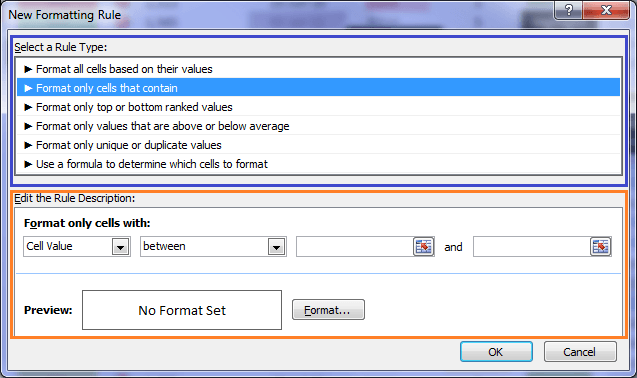
Then select the type of rule you want, and specify your criteria in the edit the rule description.
Note: Different Rule Description options will appear depending on which Rule Type you select.
Most of them are self explanatory except:
Conditional Formatting Formulas
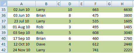
The last Rule Type in the list above is ‘Use a formula to determine which cells to format’. Basic examples of formulas you can use here are:
=$F35>500
(row 35 is the first row in my table – see example below)
This formula will apply the conditional format to all values greater than 500.
The absolute reference for column F is instructing Excel that the conditional format is dependant on column F. If you only used a relative reference for the column the formula won’t work properly.
Now, if you’ve been paying attention you’re probably thinking, why would I use a formula to format cells >500 when the ‘Greater Than’ formats are already built into the Highlight Cell Rules menu.
Well, because if you select the whole table before inserting the rule it will highlight the whole row like this:
Here's a tutorial on how to use formulas to set Conditional Formats.
For Extra Credit add Filters to your data and use the formatting as your filter criteria.


I want to apply some of the skill in my daily work as I have to sort number of records everyday and I have to generate reports – weekly, monthly and yearly.
Thank you, you just saved me hours of struggle!
Glad I could help, David 🙂
Hi I am trying to highlight the bars with respect to range of marks in my worksheet. For example marks ranging from 80-100 should have green bars marks ranging from 70-79 should have yellow bars like that. Is this possible to make. I asked one of the experts but he replied that bars formats are already pre defined and we cannot assign different formats to each desired range or value as we expect. Could you suggest on this please?
Hi Uma,
That’s correct. You might be able to use in-cell charts in a separate column to your data, as described here: https://www.myonlinetraininghub.com/excel-factor-7-in-cell-charts
If you get stuck, please post your Excel file and question on our Excel Forum where we can help you further.
Mynda
This is awesome website with great learning information. Excel is never so easy to learn until i have reached to this website.
Thanks to every one involved in providing such a learning platform. This is contributing a lot to build my skills in excel techniques.
Thanks, Nouman! Glad we could help.
Thank you for providing so much valuable information.
Thumbs up, keep it up.
Glad we could help 🙂
regarding the formula =$F35>500, how to calculate that total amounts (selected)like sum & count.
Hi Jerald,
Please use our Help Desk to upload a sample file, with detailed explanations on what are you trying to do.
Thanks for understanding
Catalin
Hi Mynda,
Is it possible to conditionally format a cell based on its font format? By font format I mean if the cell is either bolded, underlined or italic.
I’ve found a number of ways to do it using a vba macro but would like to use the ” Selection.FormatConditions.Add Type:=xlExpression, Formula1:='”=A$1=””[Single Rule]””” approach as this seems to update on user interaction.
What I’d like to do is turn the cells background to orange if the font it italic.
Many thanks
Michael
Hi Michael,
Here is a solution that does not use VBA:
Place the cursor in Sheet1 cell A1.
Go to Formulas Tab, Define Name: use the name: IsItalic, Refers to: =GET.CELL(21,Sheet1!$A1)
GET.CELL is an old EXCEL 4 Macro Function, which allows you to find a lot of information from a cell, if the cell has formula, about formatting, and so on. To check if the cell text is bold, (or the first character only!!) use =GET.CELL(20,Sheet1!$A1) in a defined name: IsBold
Note: To make the formula volatile, in order to update the results whenever excel recalculates, you can use this formula in defined name:
=GET.CELL(21,Sheet1!$A1)+0*NOW() This 0*NOW() will change the results fron TRUE or FALSE to 1 or 0, but it will provide updating.
Now, to obtain the info needed for conditional formatting, in B1 place this formula: =IsItalic When you copy this down, because the reference in GET.CELL function for rows is relative, (Sheet1!$A1), even if the formula is the same in all rows, it will work.
All you have to do now is to set the Conditional Formatting rule, with a simple reference as a formula: =$B1
Another use of GET.CEll function you can find here: https://www.myonlinetraininghub.com/excel-factor-8-highlight-cells-containing-formulas
Catalin
I am trying to use conditional formatting on an excel file that has real time data updating to it. Is this possible?
Hi Krystal,
Yes, you should be able to use conditional formatting. If you’re asking if the conditional formatting will automatically be applied to the new data then the best way to do this is by formatting your data in an Excel Table. That way the formatting rules will be copied to the new data.
I hope that helps.
Kind regards,
Mynda.
Hi,
I would need to highlight row base on a start and finish date, the row need to be highlight is based on a running date.
Example, my start date: 27-May-13 and end date: 01-Jul-13, and and i have marked the cells with running calendar date.
Please assist.
Many Thanks
Hi Chee,
I’d need to see the Excel file as you haven’t quite given me enough information. You can send it to me via the help desk.
Kind regards,
Mynda.
Hi, I am trying to use icon sets to show change as represented in a cell (C1) which has a formula =A1-B1 and represents the change between two monthly performance results, with A1 being the most recent month and B1 being the previous result. Is this possible and if so how do I set up the CF rules ???? have been searching for answers but don’t understand the CF formatting rules side of things. Why do they have 67 and 33 percent all the time and or 0’s & 1’s. Thanks David.
Hi David,
Conditional formatting icons work by comparing a value to a range of values. If the value is >=67 percent of the values you’re comparing to it will usually get a green icon, if it’s >=33 it’ll get a yellow icon and when <33 it’ll get a green icon (depending on which icon set you choose).
To tell Excel which values you want to compare to you first select them before inserting the conditional formatting rule.
I hope that helps. If you get stuck I suggest you send me your file and tell me what you’d like to see and I’ll endeavour to help you.
Kind regards,
Mynda.
Hi Mynda, I have a doubt about logical functions when I use conditional formatting.
Giving this example : = AND(A23>111)
lf I have any letter or text in the cell A23, why does excel say TRUE ?, no matter the letter or the higher the number I put, it always gives me the same answer, is considering the text as numbers ? so I wonder how excel interprets that ?
thanks
Pablo G.
Hi Pablo,
It’s sad to say that Texts are interpreted as greater than numbers.
That’s how it is.
Cheers.
CarloE
I have a worksheet which has 3 conditional formats. When I copy this worksheet as another within the same workbook (in preparation for generating some reports), I want to turn off the “Stop if True” for just the 1st of the 3 conditional formats — using VBA in my macro. Can this be done? How? Thank you very much. RogerEP
Hi Roger,
Can you please send me your workbook so I can see what you have done and work out a solution for you.
You can use the Helpdesk to create a ticket and attach a workbook to it.
Regards
Phil
Hi,
I’m wondering if there is a feature in Excel that allows me to use Icon sets in one cell with the data from another cell.
This is what im struggling with.
‘Sheet1’!A1 Name
‘Sheet2’!A1 Number from 0-10
‘Sheet2’!A2 Number 0 or 1
I would like to to use X!V icons.
If Sheet2 A2 is 1, the Icon shown in Sheet1 A1 should be ‘X’.
If Sheet2 A2 is 0, and Sheet2 A1 is between 5-10 the icon shown in Sheet1 A1 should be ‘!’
If Sheet2 A2 is 0, and Sheet 2 A1 is between 0-4 the icon Shown in Sheet1 A1 should be ‘V’.
Br Lars
Hi Lars,
You could do this with a nested IF statement with the AND function like this:
I hope that helps.
Kind regards,
Mynda.
Thank you,
But I wasn’t actually looking too use “X”, “!” and “V” as data in Sheet1 A1. I have already predefined the data in this cell. I want to use Icon set (X,!,V) as an indicator of something happening in another cell without changing the predefined data in the cell.
Lars
Hi Lars,
Excel Conditional Formats doesn’t allow you to create custom icon sets, an alternative is use another cell to generate your ‘custom icon’ using the IF function I suggested.
Kind regards,
Mynda.
mam, i search all website for excel bu i can’t learn corretly, plse tell me hot learn formulas in excel, i am a dataentry operator, i have 5 year experience, but i do not no very well excel. pls help me.how to learn easaly for vlookup, pvote table and formulas for excel
Hi Lokesh,
You can find a list of Excel Formulas here, including PivotTables and other Excel tools.
Kind regards,
Mynda.
I’m working with a fairly large spreadsheet. In order to focus on the data one row at a time, is there a way so that once a cell is clicked/selected the entire row is highlighted? and revert to no fill once it’s on another cell?
Thank you!
Hi Anita,
Great question, but a long answer. You can do it using a combination of Conditional Formatting and VBA. I haven’t written a tutorial on how to do it yet but if you send me your file I can insert it for you.
To send me your file log a ticket on the help desk.
Kind regards,
Mynda.
Please help. I have a column of numbers, day 2 copies day 1 until an actual number is received. I would like the conditional formatting to highlight the cell once hardcoded with a value to keep my place in the spreadsheet. I am sure this is possible I simply cannot select the correct options can someone help?
Hi Christina,
I’m having difficulty picturing your data. Can you please log a ticket on the help desk and attach your file or an example of your data so that I can help you further.
Thanks,
Mynda.
Hi Mynda,
I’m facing a situation where I need to format the cells of one row based on another row which has percentages. For example:
Row 7 has: 1, 2, 3
Row 8 has: 40%, 52%, 118%
I need to format row 7 (put different colors) based on the corresponding row 8 value.
Any idea whether its possible, and if it is, how to do it?
Many many thanks in advance!
Hi Kholood,
Thanks for your question. You can use Conditional formatting to do this:
In cell A7 apply the following conditional format formula (Conditional Formatting on the menu > New Rule > Use a formula to determine which cells to format):
Insert this formula:
=A8=40%
Then set your colour
Then do another one for 52% in cell A7:
=A8=52%
Then another for 118% with another colour:
=A8=118%
Then copy the format from cell A7 to cells B7 and C7.
I hope this helps.
Kind regards,
Mynda.