We often get asked if we can count colored cells on a worksheet, and yes you can.
You could count cells using a combination of conditional formatting, filters and the SUBTOTAL function, but I want to show you how writing a UDF (user defined function) can let you count, sum and average colored cells, in the same function.
Background Color or Conditional Formatting?
Before we get started I need to say that this UDF works only with cells that have their background (fill) color changed. It does not work with conditional formatting.
Before you start rolling your eyes, this limitation is down to Microsoft. You can use VBA to get the color of the cell if it is conditionally formatted:
CellColor = ActiveCell.DisplayFormat.Interior.Color
This works fine in a Sub. But put that same line into a function, and you get a #VALUE error returned.
Why? Ask Microsoft. Their documentation just states that the DisplayFormat property will generate a #VALUE error in a UDF.
So we'll just work with background color for now. I will write another blog post on conditional formatting and provide code that works with CF.
Function Declaration
We want to compare the color in a reference cell against the colors of a range of cells. So we must pass into the function both of these things. The function is called ColorMath.
Function ColorMath(InputRange As Range, ReferenceCell As Range, Optional Action As String = "S")
InputRange is the first argument and is the range of cells we are checking.
ReferenceCell is the cell with the color we are looking for.
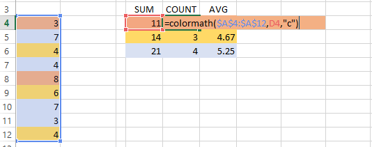
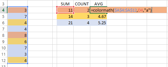
The 3rd argument is the Action we want to carry out, that is, are we going to SUM, COUNT or AVERAGE the values in the cells. This is an optional argument. If it is omitted then Action is given the default value "S" which indicates we are going to SUM values.
I've made Action a String, rather than a number as reading the formula in the sheet seems clearer to me if I see "S" for SUM, "C" for COUNT or "A" for AVERAGE. You can of course use numbers to indicate what you want your functions to do.
The string that specifies the action is not case sensitive. The function converts it to upper case before checking it.
Checking Fill Colors
The piece of code that checks the background or fill color is pretty straightforward.
The color of our ReferenceCell is assigned to the variable ReferenceColor by :
ReferenceColor = ReferenceCell.Interior.Color
Looking For The Colored Cells
Use a For ... Next loop to check each cell in the InputRange
If Action = "C" Then

  For Each Cell In InputRange

    If Cell.Interior.Color = ReferenceColor Then Result = Result + 1

  Next Cell

End If
This loop is counting the number of cells that match our ReferenceColour. The process is similar if we want to SUM or AVERAGE the matching cell values.
Some Examples
With a small list of numbers, colored as shown, I've set up my function to show me the SUM, COUNT and AVERAGE of the numbers in the three different colors.
These examples are contained in the sample workbook you can download below.
SUM
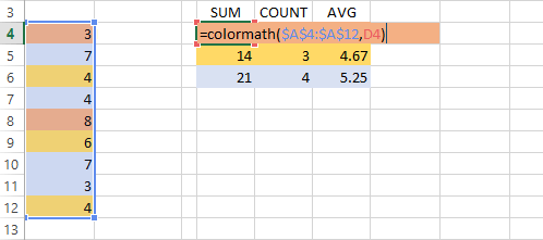
COUNT
AVERAGE
You can of course (and you should) use Named Ranges rather than specify the range as I have done in these examples.
My sample workbook uses a named range called ColoredCells.
Recalculation
If you change the fill color of a cell using the Ribbon, by right clicking and choosing Fill Color, or by right clicking and choosing Format Cells->Fill, this won’t trigger a recalculation, so a function's output may not be correct. Be wary of this.
This is down to the way Excel works. It just doesn't see a background color change as a change worthy of recalculating. Only certain things will cause Excel to recalculate.
However, using the Format Painter to change fill colors will cause a recalculation to occur.
You could also make use of the Workbook_SheetSelectionChange event to make Excel calculate as new cells are selected. Changing the fill color still won't cause a recalculation, but as soon as you click a different cell, or use the cursor keys, Excel will recalculate.
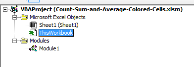
In the sample workbook below I've included code for the Workbook_SheetSelectionChange event if you want to use it.
Look in the ThisWorkbook module.
You can also make the function volatile, that is, its output is recalculated each time the sheet or workbook undergoes a recalculation.
By using the statement Application.Volatile we can make our function recalculate by pressing SHIFT+F9 to recalculate the active sheet.
Error Checking
I haven't written any specific error checking or handling routines. So if your InputRange contains a letter, you'll get a #VALUE error.
You can let Excel handle error processing, or write your own error handling routines.
Download Sample Workbook
Enter your email address below to download the sample workbook.
Download the workbook here.
To use this function, save it into your PERSONAL.XLSB or into the add-in you created after reading my last blog post.

good morning,
I have a sheet I’m creating for work that has a total number of units delivered tab and then a total hour worked tab for each employee for each day of the week.
for example, employee # 1 on Monday did 167 units in 8.58 hours but on Tuesday did 122 units in 7.62 hours
I have all the conditional formatting set to where if they have worked under 8 hours it turns yellow, between 8.01-9.49 it turns green, and over 9.5 it turns red. This formatting changes both the cell for units delivered and hours worked.
I would ideally like to average the units delivered tabs but only the ones that have turned green. I had tried a similar VBA I found online but like you said above it gives a #VALUE error because the colors are done via conditional formatting. Is there any work around to this error?
Hi Kylee,
In the same way you’ve set up the conditional formatting rules, you can use AVERAGEIFS formulas to average the data that falls into each band. If you get stuck, please post your question on our Excel forum where you can also upload a sample file and we can help you further.
Mynda
Hello
My knowledge in programing is close to null, yet this function is extremely usefull for my work.
The (probably) dumb problem I face is that if I copy my worksheet with all my data to the sample workbook you have here for download, everything works wonderfully. However, if I copy the code from your sample workbook to my personal VBAProject, in a new excel file, and I try to use the function it always gives me the error #NAME?
What’s wrong?
I have to point out that I’m working in a Mac and that my Office is in french (could that be the problem?)
Thank you
Hi Laura,
When using macro’s from personal.xlsb, you have to type “personal.xlsb!” before the UDF’s name. It’s better if you save the personal.xlsb as an add-in (.xlam file type), then activate the add-in, you will be able to use the UDF’s as regular excel functions, no need to reference the file name in function.
Catalin
Great post Philip. Is there anyway to add some descriptions or help to this function? At a bare minimum, it would be nice if the user could see what the “Action” options were.
Thanks
Hi Michael,
You can run a simple code that will register the help for that function, and will add it to a specific category from Functions list:
Sub AddFunctionDescription()

  Application.MacroOptions _

      Macro:="ColorMath", _

      Description:="Perform calculations on colored cells", _

      Category:=3, _

      ArgumentDescriptions:=Array("Input Range", "The Reference range", "Optional: Action as string. Action can be S to SUM, A to AVERAGE, or C to COUNT. If not specified the default Action is SUM")

End Sub
The categories are:
0 No category appears only in All
1 Financial
2 Date & Time
3 Math & Trig
4 Statistical
5 Lookup & Reference
6 Database
7 Text
8 Logical
9 Information
10 Commands normally hidden
11 Customizing normally hidden
12 Macro Control normally hidden
13 DDE/External normally hidden
14 User Defined default
15 Engineering only available if the Analysis Toolpak add-in is installed
This option is not available to all excel versions, just 2010 up i think.
Another option is to put all actions in the argument name:
Function ColorMath(InputRange As Range, ReferenceCell As Range, Optional OptionalAction_S_C_A As String = “S”)
After you type =ColorMath( in a cell, press Ctrl+Shift+A, this will fill all arguments with argument name:
=ColorMath(InputRange, ReferenceCell, OptionalAction_S_C_A)
There are even more complex solutions, to register the descriptions to get the Intellisense functionality, you will find one here: Excel-DNA/IntelliSense
Cheers,
Catalin
Hi Philip,
How about the other calculations like Max, or Min?
Regards,
Julian
Hi Julian,
As you already know, almost anything is possible.
But I would do things differently: instead of performing a loop for each Action, I would collect all matching cells into a range, using Union VB function, then apply any calculations to the resulting range:
Option Explicit
'
' Written by Philip Treacy
' https://www.myonlinetraininghub.com/count-sum-and-average-colored-cells
'
Function ColorMath(InputRange As Range, ReferenceCell As Range, Optional Action As String = "S")
Application.Volatile
' Action can be S to SUM, A to AVERAGE, or C to COUNT
' If not specified the default Action is SUM
Dim ReferenceColor As Long
Dim CellCount As Long
Dim Result As Variant
Dim Cell As Range, UnionRng As Range
Action = UCase(Action)
Result = 0
CellCount = 0
ReferenceColor = ReferenceCell.Interior.Color
For Each Cell In InputRange
If Cell.Interior.Color = ReferenceColor Then
If UnionRng Is Nothing Then
Set UnionRng = Cell
Else
Set UnionRng = Union(UnionRng, Cell)
End If
End If
Next Cell
If Action = "S" Then Result = Application.WorksheetFunction.Sum(UnionRng)
If Action = "C" Then Result = UnionRng.Cells.Count
If Action = "A" Then Result = Application.WorksheetFunction.Average(UnionRng)
If Action = "MIN" Then Result = Application.WorksheetFunction.Min(UnionRng)
If Action = "MAX" Then Result = Application.WorksheetFunction.Max(UnionRng)
ColorMath = Result
End Function
The average was wrong in the original code, if one of the cells has color but is empty. Using the default Average function is safer.
Thank Catalin. I was just working on modifying it to use UNION and return a range that could be used by other functions.
Good spot on the Avg error too.
Phil
Hi Catalin
Why is the Application.WorksheetFunction.Average(UnionRng) returning a #VALUE! error instead of a #DIV/0! (as in a normal Excel function would) if the cells referred to are all blanks?
Sunny
Hi Sunny,
when a UDF function hits an error, no matter what caused that error (may be a runtime error, or you have passed a string to a parameter declared as Integer for example – a mismatch), Excel will exit that function without any warning, and will return the VALUE error. In our case, we have a runtime error 1004: “Unable to get the Average property of the WorksheetFunction class”
If you disable error checking, by placing On Error Resume Next statement before the worksheet functions evaluations, the result will be 0, not VALUE or DIV/0.
A way to get the same result as the original Average sheet function is to use the Evaluate VB function:
Result= Evaluate(“=Average(” & UnionRng.Address & “)”)
This will return DIV/0 error (Error 2007 in VB)
Of course, there may be the case where UnionRng is Nothing (no cell has the selected color), the code needs to handle this situation too.
Cheers,
Catalin
Hi Catalin
Thanks for your detailed explanation.
I already saw the run time error when I tested that particular line of code (AVERAGE) via the immediate window but was just curious to know why it is like that. Normally I will try to avoid the On Error Resume Next statement unless I have to as it can cause lots of problem if misused.
Once again thanks again for your clarification.
Cheers
Sunny
Indeed, it’s better to handle errors instead of disabling them. There are cases though when you intentionally want to force an error, to see if a workbook is open for example, we even know what error number we will have:
On Error Resume NextSet Wb=Workbooks("Test.xlsx")
If Err.Number=9 then Set Wb=Workbooks.Open("C:\Test.xlsx")
on error goto 0
The Evaluate vb function will work without disabling errors, but I had a weird experience with Evaluate function, when the same function in excel sheet works and the VB Evaluate returned an error for exactly the same data. Therefore, I consider the Evaluate function unreliable.
Cheers,
Catalin
Hi Philip
Adding Application.Volatile to the code will allow recalculation when pressing the F9 key. Only drawback is it makes the function volatile.
Hi Sunny,
Yes I did think about including this but left it out. But now you have mentioned it, I have put it back in 🙂
Cheers
Phil
Hi Philip
I noticed that if you change the following line of code
Result = Result + Cell.Value
to Result = Result + WorksheetFunction.Sum(Cell)
your function will no longer trigger an error when you enter text to the cell. Any idea why this is so?
Sunny
Hi Sunny,
SUM ignores the text and only adds the numbers. You could use this, but unless you write your own code to check the input range for errors, you may not get any indication that there is an invalid cell.
I guess it’s up to the individual how they want to program.
Cheers
Phil