Last week I received the following question from André:
“I need a formula that will count how many values in cells D4:D7 are listed in B4:B13. I don’t want to count the number of times they appear in column B, I just want to know how many values from column D are in column B“.
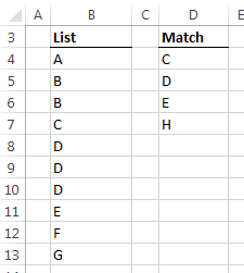
Here is the data:

The answer is 3. That is values C, D and E are in column B.
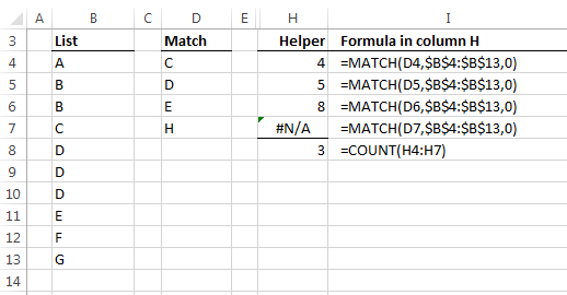
Now, we could use a helper column to check if the values in column D are in column B, and then count those that returned a match like this in column H:

There’s nothing wrong with helper columns. In fact they can be more efficient than using array formulas.
However, if you want a formula challenge then go ahead and see if you can write a formula that will return the count in a single cell. Don’t read any further until you’ve had a go yourself.
Excel COUNT MATCH Array Formula
I’m going to step through my approach, however I’m sure it’s not the only way so please share your ideas in the comments below.
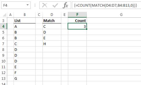
I used the COUNT and MATCH functions in an array formula like so:

Remember: array formulas are entered using CTRL+SHIFT+ENTER and the curly braces are automatically inserted by Excel.
Let’s step through how this COUNT MATCH array formula works. Here it is with colour coding:
=COUNT(MATCH(D4:D7,B4:B13,0))
The MATCH function looks up the values in cells D4:D7 and returns their position in cells B4:B13. If it doesn’t find a match it returns the #N/A error.
Normally the MATCH function looks up a single value, but because we’ve entered it as an array formula it will look up multiple values, in this case those in cells D4:D7.
When I evaluate the MATCH component of the formula it returns a list (or array) of the positions like so:
=COUNT({4;5;8;#N/A})
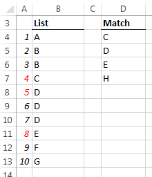
That is, C is the 4th item in the range B4:B13, D is the 5th item and E is the 8th item, as you can see below. H isn’t found so MATCH returns an error.

Note: MATCH returns the first instance of a value so the second and third instances of D are ignored. Perfect, that’s what we want.
Finally, the COUNT function simply counts how many numbers the MATCH function returns. Since #N/A is not a number it is ignored.
=COUNT({4;5;8;#N/A})
=3
Download the workbook
Enter your email address below to download the sample workbook.
Want More?
Don’t forget to share your ideas for solving this challenge in the comments below.


First, I’d love to know more about the structure of Neale’s SUMPRODUCT and why that worked.
Next, both solutions seem to be limited by the fact that column D has no duplicates. How would the formulas need to change if column D potentially had duplicate values.
Hi Jim,
In English Neale’s formula
reads:
Count the cells in B4:B13 that match the cells in D4:D7, with COUNTIF evaluated the formula now looks like this:
=SUMPRODUCT(({1;3;1;0}>=1)*1)Then test the values returned by COUNTIF to see if they’re greater than or equal to 1. The formula now looks like this:
=SUMPRODUCT({TRUE;TRUE;TRUE;FALSE}*1)Multiplying TRUE and FALSE by 1 converts them to their numeric equivalents of 1 and zero, so the formula now looks like this:
=SUMPRODUCT({1;1;1;0})And SUMPRODUCT adds those values up to return 3.
In regards to your other question about column D containing duplicates, I don’t see what the purpose of this exercise would be. If you had duplicates in both columns then what result are you trying to return?
Mynda
Thank you for the explanation of the SUMPRODUCT. That makes a lot more sense now.
As for my additional question. I’m thinking about what would happen if both lists were rather long. It would be possible to get a duplicate value in the “Match” list and not see it. Is there a way around this problem (the counts aren’t correct if there is a duplicate value in the “Match” list) or would it just be easier to always remove the duplicates from the match list first.
Hi Jim,
I’d be inclined to remove duplicates (Data tab > Remove Duplicates) before starting as opposed to trying to complicate the formula to handle them somehow.
Mynda
I avoid array formulas like the plague. I stopped using them several years ago and never looked back.
Why? Several reasons:
1) You have to use Ctrl-Shift-Enter to get the formula to work as an array formula.
2) I always forget to use Ctrl-Shift-Enter.
3) You will, too.
4) If you forget to use Ctrl-Shirt-Enter, the broken array formula does not tell you it’s broken.
5) Most normal users have no idea what an array formula is nor how not to break them.
6) Short of writing a macro (which I did), there’s no easy way to see where array formulas are, thereby making it harder to find out which one(s) you or someone else accidentally broke.
What do I use instead? The SUMPRODUCT() function! It can do almost anything (maybe everything) an array formula can do and there’s no Ctrl-Shift-Enter to mess around with.
Great points, Dave.
SUMPRODUCT is in fact a ‘modern’ array function, in that it handles arrays of data, but it doesn’t require using CTRL+SHIFT+ENTER. For those interested you can learn more about SUMPRODUCT here.
Mynda
I will use a helper column with VLOOKUP and COUNTIFS.
In cell J4 =VLOOKUP(D4,$B$4:$B$13,1,FALSE) copied down till J7.
In cell J8 =COUNTIFS(J4:J7,”#N/A”)
I will normally avoid using array formulas.
Hi Sunny,
I thought about a similar VLOOKUP solution too.
I think your COUNTIFS is meant to be:
Mynda
It looks like the symbols were auto removed when I posted them.
Ah, that would explain it.
Non-array solution
=SUMPRODUCT((COUNTIF(B4:B13,D4:D7)>=1)*1)
Seems to work OK.
Nice!
I always thought that for every array formula there was a SUMPRODUCT equivalent.
However, in this instance, the closest that I found was:
=SUMPRODUCT((B4:B13=D4)+(B4:B13=D5)+(B4:B13=D6)+(B4:B13=D7)*1)
– which produces a result of 5, being number of instances of Match values appearing in the List values.
In some cases this would be more useful, but it is obviously not the same as returning a count of how many of the Match values appear in the List values.
Is there a SUMPRODUCT equivalent for this problem?
Hi Stephen,
Thanks for having a go. Neale’s SUMPRODUCT version works.
Cheers,
Mynda
Excellent!
I knew that there had to be a SUMPRODUCT solution there somewhere. 🙂
I have replied to you personally this past week, but let me thank you again in this forum for helping me with my query , and quickly too! André
🙂 my pleasure, André