The SUMPRODUCT function is one of Excel's most versatile functions.
But now that we have SUMIFS, COUNTIFS, AVERAGEIFS etc. it’s easy to think this function is, dare I say, redundant!
However, SUMPRODUCT can do things you can’t do with those functions.
Table of Contents
Watch the Video

Download Workbook
Enter your email address below to download the example files.

Introduction to the SUMPRODUCT Function
In its simplest form the SUMPRODUCT function multiplies corresponding components in the given arrays and returns the sum of those products.
If you have two arrays of numbers, it will multiply each pair and then sum up those results.
The syntax for SUMPRODUCT is
=SUMPRODUCT(array1, [array2], [array3], ...)
Where array is the range of cells you want to multiply. Note: arrays must be the same size.
SUMPRODUCT Function Practical Examples
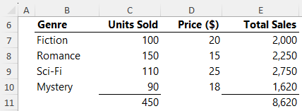
Imagine you run a small bookstore. You have various genres of books, each sold at different prices, and sold in different quantities each month. Our data set for the month looks like this:
Let's navigate through the different scenarios of SUMPRODUCT using this dataset.
Basic Use of SUMPRODUCT
To find out the total revenue for the month, we'd multiply the units sold of each genre by its price, and then sum those up using this formula:
=SUMPRODUCT(C7:C10, D7:D10)
Which evaluates to:
=SUMPRODUCT(

{100;150;110; 90},

{20;15;25;18}

)
Each array is multiplied by the other like so:
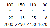
And the result of each sum is then added up, resulting in:
=8,620
Using SUMPRODUCT is a breeze and importantly, doesn’t require the intermediate steps in column E.
SUMPRODUCT with AND criteria
Let's say you want to find out the revenue for books that are priced above $15 AND sold more than 85 units.
We can use logical tests inside SUMPRODUCT to identify which rows to include in the array!
This is similar to SUMIFS, except you don’t need the intermediary values in column E first.
Using the formula below, we can find the total sales of books where the Units Sold is > 85 AND the Price is > $15:
=SUMPRODUCT((C7:C10>85)*(D7:D10>15), C7:C10, D7:D10)
Here, the logical tests return arrays of TRUE and FALSE values:
=SUMPRODUCT(

{TRUE;TRUE;TRUE;TRUE}

*

{TRUE;FALSE;TRUE;TRUE},

C7:C10,

D7:D10)
And when a math operation is applied to them, in this case multiplication, they convert to their numeric equivalents of 1 and 0 (zero):
=SUMPRODUCT(

{1;0;1;1},

C7:C10,

D7:D10)
These 1s and 0s are multiplied by the other two arrays, thus eliminating any values in the corresponding arrays that don’t meet the criteria.
=SUMPRODUCT(

{1;0;1;1},

{100;150;110;90},

{20;15;25;18}

)
SUMPRODUCT with OR criteria
Now, what if we want to calculate the revenue for books priced above $20 OR sold more than 100 units?
There are two changes required: we use the addition operator (+) to achieve the OR functionality.
And to avoid double counting records, we must wrap the logical tests in the SIGN function.
The SIGN function returns 1 for a positive value, zero (0) if the number is 0, and -1 if the number is negative. Your SUMPRODUCT formula would look like this:
=SUMPRODUCT(SIGN((C7:C10>100) + (D7:D10>20)), C7:C10, D7:D10)
Evaluating the logical tests results in row 3 returning TRUE for both logical tests:
=SUMPRODUCT(

SIGN(

{FALSE;TRUE;TRUE;FALSE}

+

{FALSE;FALSE;TRUE;FALSE}),

C7:C10,

D7:D10

)
And when those tests are added together it results in 2 for the third row:
=SUMPRODUCT(SIGN({0;1;2;0}), C7:C10, D7:D10)
Without intervention, this would result in double counting the sales for Sci-Fi. But with the SIGN function, all positive values in the array are converted to 1, resulting in the correct calculation:
=SUMPRODUCT({0;1;1;0}, C7:C10, D7:D10)
SUMPRODUCT Single Logical Tests
As the months roll by, you keep track of the sales of each genre by date. Suppose for a particular month, your data now looks like this:
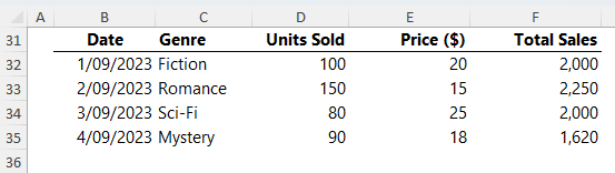
To find out the revenue for books sold after the 2nd of September we can use the following formula:
=SUMPRODUCT( -- (B32:B35>DATE(2023,9,2)),D32:D35,E32:E35)
The DATE function helps us specify the criteria date and because there is no math operation being performed, we use the double unary (two minus signs) to coerce the Boolean logical tests into their numeric equivalents of 1 for TRUE and 0 for FALSE.
Note: there is no space between the two minus signs in the double unary in the formula. If you can see a slight gap, that's just the way the font is displayed on yoru screen.
The formula evaluates like so:
=SUMPRODUCT( -- ({FALSE;FALSE;TRUE;TRUE}),D32:D35,E32:E35)
And when the double unary is applied it returns:
=SUMPRODUCT({0;0;1;1},D32:D35,E32:E35)
SUMPRODUCT as an alternative to COUNTIF
Say you want to find out how many genres' book price is less than $20.
We don’t need to aggregate any values from the table, but rather just count the number of logical tests that return TRUE resulting in a simpler formula:
=SUMPRODUCT(--(D7:D10<20))
Again, the double unary coerces the TRUE and FALSE results to their numeric equivalent for SUMPRODUCT to aggregate:
=SUMPRODUCT({0;1;0;1})
SUMPRODUCT as an alternative to AVERAGEIFS
You're curious about the average price of books sold in quantities greater than 100 units.
=SUMPRODUCT(--(C7:C10>100),C7:C10,D7:D10)/SUMPRODUCT(--(C7:C10>100),C7:C10)
The numerator gives us the total price of books that meet the criteria, and the denominator gives the count of such books. Dividing them gives the average.
Quick Recap, Rules, and Limitations
In SUMPRODUCT functions you can employ the AND logic, and OR logic using the * and + symbol:
- When the multiplication symbol * is used it reads ‘AND’.
- When the plus symbol + is used it reads ‘OR’.
- If the OR criteria reference different columns, you should wrap the logical tests in the SIGN function to avoid double counting.
- If you only have one logical test, use the double unary to coerce the Boolean TRUE and FALSE values to their numeric equivalents.
- Each array referenced in SUMPRODUCT must always be the same size.
- Text values included in arrays referenced by SUMPRODUCT will be treated as zero.
- SUMPRODUCT can be resource-intensive, especially with large data sets - see below for alternatives.
SUMPRODUCT Function Benefits
The SUMPRODUCT function is a powerhouse! It's versatile, efficient, and can replace many other functions when used creatively.
We hope our bookstore example shed light on its applications. Next time you find yourself reaching for a SUMIFS or AVERAGEIFS, consider giving SUMPRODUCT a shot!
SUMPRODUCT Performance
While SUMPRODUCT is a power horse of a function, users with Excel 2021 onward can achieve similar results with the newer FILTER function. FILTER enables you to extract the data you want to aggregate and may be more efficient over large datasets.

How to use the SUMPRODUCT function for converting monthly data into quarterly totals?
Hi Nirmal,
Please see this tutorial on converting monthly data into quarters.
Mynda
Giving some numbers in date format in range B453:I453, as well as another number in cell A455, I tried to count the number of days meet the criteria, The first formula to test the WEEKDAY is ok, while the second formula just returned an #VALUE! error. I replaced the WEEKDAY with MONTH and it still worked. Could you please tell me what’s the problems with WEEKNUM. By the way, it seems that CSE formula can’t take this way like {=WEEKNUM(B453:I453)} referring the days in the range as mentioned above.
=SUMPRODUCT((WEEKDAY(B453:I453)=A455)+0)
=SUMPRODUCT((WEEKNUM(B453:I453)=A455)+0)
WEEKNUM can’t take an array or range in it’s first argument, whereas WEEKDAY can. You could use the BYROW function to test each row for the WEEKNUM e.g.
Mynda
It has been confusing me for long. Now that with your affirmative answer I should not waste time to try it that way again and again. Thank you for the valuable information.
Pleasure
Don’t get me wrong when I ask this because I am a huge fan and longtime user of SUMPRODUCT all the way back to the days before Microsoft started offering the “S” forms of COUNTIF etc. (because back then, it was the only way to handle multiple conditions without CSE arrays). I’m actually just curious to get your opinion.
While I will probably never call SUMPRODUCT entirely obsolete or redundant, do you think Excel 365 and its FILTER function have largely provided the opportunity for it to cash in a well-earned retirement? Using a SUM(FILTER…)) formula would give the same result and require the same implementation of logical tests, or what I think of as binary logic, that are multiplied or added together. But this approach also offers the ability to calculate MEDIAN(FILTER(…)) or QUARTILE(FILTER(…)) or others.
Yes, when used creatively and properly, AGGREGATE could handle those two situations and a few others, but what about things like GEOMEAN(FILTER…))?
Yes, absolutely, David. I would use the FITLER function over SUMPRODUCT most of the time, assuming I didn’t need the file to be backward compatible with Excel 2019 or earlier.
Dear Mynda Treacy,
Thank you so much for providing this information.
As a user of Excel 2000 SUMIFS is not an available function.
I tried using Microsoft’s online version of Excel to see if SUMIFS would work which it did, but I need access to a macro or two which are not available.
On a hunch I searched for an alternative to SUMIFS and up popped your article.
I have to say, there are a lot of people out there who could take a lesson from you on how to properly present information in a manner that is thorough, easy to read and easy to understand when it comes to Excel.
Your inclusion of Using Dates as Criteria, helped me immensely in using a Date, drop-down list to provide yearly summary information.
Thank you again.
Regards,
-Kevin N.
Thanks for your kind words, Kevin! I’m so pleased this tutorial was helpful.
Mynda thank you so much for creating this resource.
The fact that your post is useful even after 10 years from the time you published speaks of its value.
I like your presentation style; the way you decompose formula syntax in plain English with decently spaced brackets and signage. Makes it easier to understand and grasp.
I was stuck with converting a SUMIFS into SUMPRODUCT involving references to an external workbok (you know how SUMIFS stops to render results when external workbooks are closed/ not opened). This post helped me crack the right code within minutes.
Cheers!
Nevill
Thanks for your kind words, Nevill! I’m delighted you found this tutorial helpful 🙂
Many thanks for this, really helpful.
One of the things i noted is that it gives an error if there is a cell without a number, whereas SUMIF still works. For example in my dataset instead of zeroes I have “N/A” which should be ignored. The sumif still works and ignores these but sumproduct doesn’t and given an error, is there anyway around this using sumproduct?
Hi,
try the AGGREGATE function, this one can ignore errors easily.
Very many thanks for developing us to be more efficient in our work place.
Glad we can help, David 🙂
hay there, thanks for sharing very helpful examples. i just wanted to know if i could use Sumproduct formula with reference values but not the complete values.
Example: i have different part descriptions like: Air filter, Oil filter, cabin filter, disk pads, spark plugs and i want to sum only having word “Filter”.
Can you please help me in this.
Thanks
Hi Muhammad,
Try this one:
=SUMPRODUCT((ISNUMBER(SEARCH(“filter”,A1:A6)))*1)
Catalin
I am interested in Pre-2007 versions of Excels COUNTIFS() and SUMIFS() so that the application I am working on will be backwardly compatible.
Amazing.. Very much helping to achieve the results with one formula for all the need of COUNTIF, SUMIFS etc. Thanks for enlightening this.
Thank you,
This has solved my compatibility issues that were breaking lookups between Excel 2013 and 2010 sheets.
In a comment from April 8, 2013, Bob Phillips noted this nuance in a reply to Justin, but the “why” wasn’t really explained. As Mynda has shown, a + is used for OR conditions, but if those conditions are being evaluated on different columns, then it’s possible for two or more of them to be true, causing the 1 (TRUE) results to add up to a value greater than 1. This would obviously ruin the count/sum trick, so a SIGN should be used to address that potential.
Say we needed to count the number of orders where bid = Sell or solarSystem = Rens. We would not want to double count orders that are both Sell and Rens, so the safest formula would be as follows:
=SUMPRODUCT(SIGN((bid=”Sell”)+(solarSystem=”Rens”)))
GOOD MATERIAL
Thanks! Glad you found it useful.
I’ve been struggling with the limitations of SUMIFS for years, but this solved my problem. I don’t believe SUMIFS can do >a certain cell for the criteria, but SUMPRODUCT can. Thank you!
Mynda, great article! Thank you! It explains a lot 🙂
is there any function or formulas to find out the name of the centre where pt’s surgery was done.
fox ex. a pt visited at centre A but was operated in centre B. now I have find out the total sum by using sumproduct or sumifs function for same I want to know in which centre pt was operated from a database.
Hi,
Can you prepare a sample file with your data structure? This way I will be able to give a personalized answer. You can use our Help Desk System, to upload the sample file:
https://www.myonlinetraininghub.com/help-desk
Cheers,
Catalin
Hello,
To practice sumproduct function, I set up the same the table you are presenting here. I created range name for the columns and copied the same formula you have up here. for any reason, I am getting VALUE error. Can you please explain where I went wrong that I am facing this error?
Thank you so much for your help,
Maryam
Hi Maryam,
First of all, make sure your named ranges are of equal size. If they are then check for blanks in your data ranges.
If it’s neither of those then we’ll need to see the file, which you can share via the Help Desk.
Kind regards,
Mynda
Thank you so much for your quick response. I will check on those criteria and if the issue still exists, I will send you my spreadsheet thru help desk.
Regards,
Maryam
You are awesome! this function helped me to automate a forecast sheet at my work.
Thank you for introducing and explaining all these Excel capabilities.
Maryam
Hi Maryam,
Thanks for your kind words 🙂 Just glad I could help.
Mynda
Hi, this is nice illustration of sumproduct. But, suppose, i am having abcd columns. B and d contains the amount to be totalled, based on a and c, which contains the codes for those amount. I want to use this formula, to sum all the identical matches in a and c column which contains some specific codes.
if suppose, a1, a5, c2,c13,a12 has the same code, say iia, then i want to sum up the amount in b and d columns only matching the code in a and c. how to go around to work this. Expecting your reply, as promised above in your link to comment
Hi Jraju,
Please upload to Help Desk: https://www.myonlinetraininghub.com/help-desk a sample workbook with your data, it will be easier for us to understand your situation.
Catalin
Realy Good contents & very useful tips are available in this site.
Thanks Jawa
mynad dear
good website your .mr30 ,thanks
Thanks, Mano 🙂
Nice! Thanks for explaining it clearly
you are a great women
Thank you, Haider 🙂
Hi Mynda,
Thank you for this great trick!
I am struggling right now with OR in different columns, i.g:
A B C
$10 1 1
$20 5 2
$15 2 1
I´ll need to sum all the money with B < 2 OR C < 2, so I´ve tried the following:
SUMPRODUCT((A1:A3)*(B1:B3<2)+(C1:C3<2)), that means:
SUM (MONEY IF (B<2) OR (C< 2)), so it will sum the first row and third row, that means $25, but I always get $12.
Thank you for your help
Hi German,
The OR operation is designed to allow multiple criteria in the same column. Once you start referencing criteria in other columns it only works if both criteria cannot be true at the same time which is not the case for the $10 amount where both columns B and C are less than 2.
Instead you can use this formula to achieve what you want:
Entered with CTRL+SHIFT+ENTER as it's an array formula
Kind regards,
Mynda.
Hi,
I have been struggling with the below, I think SUMPRODUCT might help, but I am unable to make it work, please suggest:
I have an employee database with salaries in multiple currencies. I need to classify salaries into fixed bands A, B, C, D. Further, the bands are different for different currencies. As of now, I have 5 currencies, so the IF statement has become a unwieldy.
The data looks something like this:
Name Currency Salary Band
EMP1 USD 6250
EMP2 USD 3300
EMP3 EURO 3673
EMP4 EURO 10167
There are four bands, e.g. for USD, they are
USD-A: 8000
How can I fill up the band using a formula
Thanks
Hi Pankaj,
You need VLOOKUP with a sorted list for this.
Kind regards,
Mynda.
This really helped a lot. I had a query regarding the sumproduct function. Could I mail u the worksheet ?
Hi Sheena,
You can send worksheets and questions via the help desk.
Kind regards,
Mynda.
thanks for quick the reply Mynda. Ive also sent the worksheet via helpdesk.
The problem basically is to use the sumproduct function in excel to add multiple columns with reference to multiple criteria in multiple columns. A rough example is given below:
Color1 weight1 Color2 Weight2 Color3 Weight3 Color4 weight4
white 280 white 48 indigo 56 red 23
red 34 indigo 25 Blue 65 red 32
Blue 23 red 51 Blue 89 indigo 51
Blue 272 orange 35 orange 40 Blue 27
i want to sum all the weight columns which are with reference to specific colors in all the color columns.
For example if i wanted to find out the total weight with respect to the colour “Blue” the desired result should come up to be 476 that is adding the values 23+272+65+89+27. similarly if i wanted to find out the total weight with respect to the color “white” the desired result should be 328(280+48), adding the corresponding values in weight column.
what would be the required sumproduct formula for this situation?
Hi Sheena,
You can use this SUMPRODUCT formula where your data above is in A1:H4:
The logical test (A1:G4=”Blue”) checks for Blue in columns A:G.
The double unary, that is the two minus signs before the logical test –(A1:G4=”Blue”), convert the TRUE/FALSE results into their numeric equivalents of 1 and 0.
So your formula looks like this after the logical test:
=SUMPRODUCT(({0,0,0,0;0,0,1,0;1,0,1,0;1,0,0,1}),(B1:H4))Because the range to be summed (B1:H4) is offset by 1 column, i.e. it starts in column B as opposed to column A like the logical test, the values form an array that matches the test with the corresponding value like this (note: the two arrays are still the same size even though they are offset):
=SUMPRODUCT(({0,0,0,0;0,0,1,0;1,0,1,0;1,0,0,1}),(280,48,56,23;34,25,65,32;23,51,89,51;272,35,40,27))SUMPRODUCT then multiplies the arrays:
And you get 476
I hope that helps.
Kind regards,
Mynda.
Hi Mynda,
Sorry I am late in the party, Thanks for making Sumproduct formula easy to understand.. till now i hv understood that we use ‘+’ sign as an OR and ‘*’ sign as an AND operator in Sumproduct formula.
I have seen many people use ‘- -‘ in a sumproduct, will appreciate if you can explain the use and why it is used please ?
Thanks in advance
Pradeep
Hi Pradeep,
The double unary ‘- -‘ is used to convert the boolean TRUE/FALSE to their numeric equivalents of 1 and 0.
Kind regards,
Mynda.
Thanks Mynda..
i got it.. but little unsure… a small example will help… may be in your next blog, or else u can write a next one to explain..
Thanks for all your help.
Pradeep
Sure, maybe next time.
Can you also please demonstrate how can we use SUMPRODUCT for getting the top 5 with multiple critera’s for e.g.
I need to know the sum of the top 5 Volumes for SolarSystem ‘EndRulf’ and jumps = 6 (considering there are 2,3,4,5.. jumps)
Hi Acpt,
Like this:
Kind regards,
Mynda.
truly a great lesson, I had a computer course and I also give lessons on excel, and this website provides the motivation for me. thank you for sharing. Greetings TCC Sampit.
You’re welcome, TCC Sampit 🙂
I have gone through your excel formula,and i found it is very useful tool .
Thanks, Gautam 🙂
Could you please help me? I have used SUMPRODUCT in a 2007 sheet as the file has to be used on a PC which has Excel 2003. However, I keep on getting the #NAME! error and, for the life of me, I can not see why. Are you able to see what is wrong with
=SUMPRODUCT((‘Referral Progress’!$D$1:$D$8197=’Area Overview’!$A4)*(‘Referral Progress’!$J$1:$J$8197>=’Area Overview’!K$1)*(‘Referral Progress’!$J$1:$J$8197<'Area Overview'!T$1))
Thank you in advance
Hi Seth,
I would like to inform you that I don’t have 2003 anymore.
However, Let’s see what we can do. Please send that file via HELP DESK.
Cheers,
CarloE
I’ve been playing with the fomula for a bit and kind of got it figured out but when I add more rows of data to imput it is not picking them up even though the data is in the ranges. On one worksheet is a log where I am entering the data as it comes in. On the next worksheet is a summary that spreads the data into groups that are easier to compare and figure out issues/problems. Right now my formula looks like this “=SUMPRODUCT((‘2013 Crane Repair Log.xls’!Date>=B19)*(‘2013 Crane Repair Log.xls’!Date<=C19)*('2013 Crane Repair Log.xls'!CraneNumber="15")*'2013 Crane Repair Log.xls'!Value)" Date CraneNumber and Value are all ranges I've created. Please help!
Hi Chris,
Try reading Array Formulas.
Or you might send your file to Help Desk.
Cheers.
CarloE
Or use dynamic named ranges.
Hi,
I have a data where i have put the date like 01.02.2011,13.02.2012.
but when i am going to apply date formula then i am getting 01 and 13 as a month but i want 02 as a month so please give me a formula to apply here.
Hi Dusmanta,
I think all you need to do is to format your cells.
Right click the cells where your dates are and
1 Format Cells
2 This will bring you to the Number’s tab
3 Select Custom -> “mm/dd/yyyy”
Please read more on formatting cells.
Now you may not find an exact format :mm/dd/yyyy.
Just choose the closest or any custom date
format for that matter and manually edit the same
to mm/dd/yyyy.
Cheers.
CarloE
Hi Mynda,
Wonderful explanation, thank you! I literally spent days searching for the right formula for my spreadsheet and this is the only site which made me understand why SUMPRODUCT would work, instead of copying/pasting formulas found online.
My formula doesn’t seem to be adding up properly though. I have the following:
Date Budget Amount
01/01/13 Stationery 12.00
02/01/13 Expenses 5.00
07/01/13 Entertainement 7.00
I want to see how much I’m spending per budget and per week (for instance Expenses from 1 Jan-7 Jan) so I used:
=SUMPRODUCT(amount,(budget=”Expenses”),(date>=DATEVALUE(“01/01/13”)),(date<=DATEVALUE("07/01/13"))) but I keep getting 0 instead of 5 as a result. Would you have any advice on what I'm doing wrong?
Hi Lisa,
Please use this formula.
=SUMPRODUCT((Amount)*((Budget="Expenses")*(AND(Date>=DATEVALUE("01/01/2013"),Date<=DATEVALUE("07/01/13")))))Assumptions: Named Ranges: Budget, Date and Amount
Read More: Sumproduct
Cheers.
CarloE
Ooops sorry something went wrong in my comment.
I meant to say I used the formula =SUMPRODUCT((amount)*((budget=”Expenses”)*(AND(date>=DATEVALUE(“01/01/13”); date=DATEVALUE(“01/01/2011″)*(Date<=DATEVALUE(“31/01/2011″))))?
Thanks again;
-Lisa
Hi Lisa,
I don’t know if it is already working or not, judging on how you wrote your feedback. 🙂
Anyway, Just send your concern via HELP DESK.
Cheers.
CarloE
Thanks Carlo, I send the details to the Helpdesk. 🙂
ARe you sure that formula works. I don’t think it does, because the AND will return a single TRUE/FALSE result, not an array of TRUE/FALSE that evaluates those date conditions.
This works perfectly fine
=SUMPRODUCT(–(Budget=”Expenses”),–(Date>=–(“2013-01-01”)),–(Date<=–("2013-07-01")),Amount)
I would also advise using this ISO standard date format to remove any ambiguity as to what the date being tested actually is (is 01/07/2013 7th Jan or 1st July?).
Hi thanks for the useful info above. I would be grateful if you could help me with my following query:
i have text name in Column A and i want to sumproduct values in column B & C with reference to specific names under Column A. Is this possible through sumproduct formula ?
Hi Gaurav,
Greetings.
Yes you can… very much.
Try this example.
Assume the data
    A       B     C
1 Names	 Value1 Value2
2 Name1	   10	  10
3 Name2	   20	  20
4 Name3	   30	  30
paste this formula anywhere in the sheet.
Please read more on SUMPRODUCT.
Cheers.
CarloE
Carloe…
I dont know how should i express my gratitude to you. The formula really works and this is a simple solution to my complex problem. I am amazed on how do you extend your support to someone, whom you dont even know!!! Thanks for your assistance, god bless you !
Regards
Gaurav Sahni, India
Hi Gaurav,
On behalf of Mynda and Philip, I say You’re Welcome!!!
It always feel good to have someone appreciate ones work too.
So thank you too.
Cheers.
CarloE
You don’t need to do the multiply in the formula, SUMPRODUCT does the multiply (PRODUCT), so you can use
=SUMPRODUCT(–(A2:A4=”Name1″),B2:B4,C2:C4)
which will also handle text values in the sum ranges as mentioned elsewhere.
Hi, Carlo.
Thank your for your answer.
I discover myself, today, the solution:
=SUMPRODUCT((Volume)*(ISNUMBER(SEARCH(“E”, LEFT(solarSystem, 1))))*(jumps=6))
But it is wrong this: =SUMPRODUCT((Volume)*(ISNUMBER(SEARCH(“E*”, solarSystem)))*(jumps=6)) because function ‘SEARCH’ search for character ‘E’ in all word, not begin with character ‘E’.
Can you explain me, please, why when evaluate, for example (jumps=6), sometimes return a list like {1,0,1,0…} and sometimes return a list like {TRUE, FALSE, TRUE, FALSE…}.
Thank you very mutch.
Sorry Mynda for ‘i’.
Best regards,
Sorin.
Hi Sorin,
Glad you found a solution. Well done 🙂
When SUMPRODUCT evaluates the jumps=6 criteria it returns an array of TRUE’s and FALSE’S. In Excel a TRUE = 1 and FALSE = 0. The multiplication before the argument *(jumps=6) coerces the series of TRUE’s and FALSE’s into 1’s and 0’s.
The multiplication does the same as the double unary in this formula –ISERROR(SEARCH(“Rens”, solarSystem)))
More on array formulas here.
I hope that helps.
Kind regards,
Mynda.
Hi Sorin,
Please send your file to HELP DESK so we can understand what you are trying to do.
My apologies I wasn’t thinking of a SEARCH function when I said you can use equal(=) and asterisk(*) to simulate a LIKE function in
programmming. Anyways, SEARCH function don’t need asterisk or any wildcard character like a question mark(?) for it to function as it does.
It’s like a ‘LIKE’ function only within a TEXT.
On this note, I am confused. Why would you want to simulate an “E*” wildcard search?
Are you trying to validate whether a word begins with a letter E?
You could just use LEFT(Word,1)= “E”.
perhaps a formula like this:
Anyway, I’m still not quite sure as to what you really want here. So might as well
send your file through HELP DESK.
Sincerely,
CarloE
Hi Mynda,
Thank you very much for explanations. This explain a lot. 🙂
Yes Carlo, it is very simple your solution, but some times we don’t find a easiest solutions.
I post the solution I was find, not best solution. Thank you for support.
Best regards,
Sorin
Hi Sorin,
On behalf of Mynda and Philip, you’re welcome.
Cheers.
Carlo
Hi Minda,
Very nice and very useful.
Thank you very much for explication and for all hard work.
I wonder how can I implement a condition “like”. It is possible?
For example: =SUMPRODUCT((Volume)*(solarSystem like “E*”)*(jumps=6))
I discover another useful criteria; if you wont to skip some records:
=SUMPRODUCT((Volume)*(–ISERROR(SEARCH(“Rens”, solarSystem)))*(jumps=6))
In this example the sum skip the records “Rens”.
I hope this help.
Best regards,
Sorin.
Hi Sorin,
I never thought you were asking a question. Sorry. 😉
Anyways, in a formula level I don’t think you can use ‘Like’ like
you can use an ‘And’ or an ‘Or’.
With you asking that, I suppose you know about programming like VBA.
Well, it’s where you can use the operator ‘LIKE’. However, in a formula level the
combination of an equal sign (=) and an asterisk (*), will give
you the effect of a like operator.
So why don’t you send your file and let us see what you want to do so we can
help via HELP DESK.
Cheers.
CarloE
Combine the LEFT function to get what you want
=SUMPRODUCT(–(LEFT(solarSystem,1)=”E”),–(jumps=6),volume)
Hi
I would like to calculate the sum of all values in a range which are NOT equal to the criteria of two values (each of which are in different ranges).
So the ranges are as below:
R1 R2
1 2
1 3
1 4
2 2
2 3
1 2
2 4
2 6
2 4
So, if the value in R1 is 1 and the value in R2 is 2 calculate the sum of the values remaining in R1.
So there are 2 rows where R1 is 1 and R2 is 2.
Adding up the remaining values in R1 gives a total of 12.
How do I calculate the answer 12?
Another example from the ranges above is
Calculate the sum of all values remaining in R1 after the following is met:
R1=1 and R2=2
AND
R1=2 and R2=4
Answer is 8
Many thanks for your help!!
Dear Justin,
Quite a brain twister you’ve got there. I don’t know why SumIF or SUmproduct alone won’t work using “<>“(not equal) conditions.
Instead of an “AND” effect, it is more like getting an “OR”
so I improvised: Note : Row1 and Row 2… columns A to I.
this will result to 12.
this will result to 8
I would like to point out in this second formula that you could have not meant AND It’s clear that it’s an OR
because you can’t have 4 conditions on two parallel cells being evaluated.
hence; OR(AND(r<>1,r<>2),AND(r<>2,r<>4). So it’s a plus(+) and not an asterisk(*)
I hope you’ll like it.
The logic is simple. I added first all in row 1. So the total is 14.
Then,
I used SUMIFS and SUMPRODUCT respectively to get the supposedly numbers to be excluded
and deducted it from the total.
Read more on SUMIFS and SUMPRODUCTS
Sincerely,
Carlo
Or you could use
=SUMPRODUCT(SIGN((A2:A10R1)+(B2:B10R2)),A2:A10)
Thanks, a very informative explanation. One question, lets say I have to sum a range based on thee AND statements and one OR, for performance would it be better to use the SUMPRODUCT as you describe, or to add two SUMIFS?
Hi Peter,
I’d choose SUMPRODUCT, but if you feel more comfortable with the SUMIFS then go with that.
Kind regards,
Mynda.
Hi
Very well explained. i only use Excel once in a while, and many features get lost over time. So your kind of assistance is a great help, when need arise.
regards
Otto Nielsen
Denmark
PS: And I am human …I think
🙂 cheers, Otto.
Thank u, I was searching for this solution
Hi,
Thanks for your detailed explanation however could you please send some more exercise to practice on
Thanks in advance.
Regards,
Vicky
Hi Vicky,
If you want to join my Excel course you receive Excel workbooks with homework questions for practice.
Kind regards,
Mynda.
kudos,excellent work
Thank you, Joseph 🙂
Hi Mynda,
Thanks Mynda for such a clear explanation of function.
🙂 You’re welcome.
Thanks for this. Now I understand well the power of SUMPRODUCT…
You’re welcome, Marlo 🙂
i need to ask a question on this…
i have an excel sheet which contains my problem…how can i attach it…
Hi Nurzy,
You can send me files by logging a ticket on the help desk.
Kind regards,
Mynda.
I don’t know if it’s just me, but I tried what you suggested and had an error but found out what was wrong. Instead of
=SUMPRODUCT((Volume)*((solarSystem=”Endrulf”)*(jumps=6)))
it should be
=SUMPRODUCT((Volume),((solarSystem=”Endrulf”)*(jumps=6)))
Use a comma instead of asterisk after the array you want to sum. Just FYI.
Hi Elton,
Thanks for your comment. Both methods give the same result for me.
Kind regards,
Mynda.
Hi,
While both formulas are valid, I’ve found that using Elton’s formula can be useful where the range you are summing contains text (e.g. headings). This can be useful when you are progressively adding to a dataset and so want to sum whole columns.
For example:
=SUMPRODUCT((D:D)*((G:G=”Endrulf”)*(H:H=6))) would result in a #VALUE! error due to text in the column headings
but
=SUMPRODUCT((D:D),((G:G=”Endrulf”)*(H:H=6))) will give you the correct result (being 44,463,091).
You need to have at least two arguments in the second array or the formula will return 0. If you only have 1, you can get around it by inserting 1* e.g.:
=SUMPRODUCT((D:D),1*(G:G=”Endrulf”))
however this is a bit of a kludge.
Anyways… that’s my two cents!
Cheers, Alison 🙂
Issue:
=SUMPRODUCT((Volume)*((solarSystem=”Rens”)+(solarSystem=”Endrulf”))*(jumps=6))
This will over count if both conditions of your “or” are true. It should be
=SUMPRODUCT((Volume)*or((solarSystem=”Rens”),(solarSystem=”Endrulf”))*(jumps=6))
Hi Kenneth,
Thanks for your comment, but since Rens and Endrulf are in the same column (solarSystem) they can’t both be true at the same time therefore double counting in this instance isn’t a concern.
Also note; your formula evaluates to 654,429,777 which is the SUM of volume where Jumps = 6. It is ignoring the OR statement in the SUMPRODUCT.
Kind regards,
Mynda.
Very useful & easy to absorbe. cheers,
Cheers, Vaidehi 🙂
I am using the 2003 Excel and I am trying to use two criteria, and to add the numbers in a third column. Now I have use this method in another workbook and it worked. But with the other workbook, the criteria’s were looking for “X” in both and the adding the third column when it applied. With this new workbook, the criteria’s are both numbers, and then add from a third column. The formula wont work if both the criteria are numbers for some reason. Do you have any suggestions?
Hi Julie,
I’d need to see your formula to know what the problem might be.
Kind regards,
Mynda.
=SUMPRODUCT((ColI=”X”)*(TVCC=”X”)*Total) This is the formula that worked, I want the exact same thing but replace the “X”‘s with 5 to 9 digit numbers.
Thanks
Hi Julie,
If you replace the x’s with numbers then you don’t put them inside double quotes….unless of course they are text and not numbers. In which case you would put them inside double quotes.
Remember double quotes tell Excel the data is text not a value/number.
If you can’t get it to work you’ll need to send me the workbook so I can see the data you’re working with.
Kind regards,
Mynda.
That was it! Thank you very much Mynda, that was very helpful. I forgot about that rule with the quotes.
I really appreciate the quick responses aswell.
Best wishes,
Julie.
You’re welcome, Julie 🙂 Thanks for letting me know you sorted it out.
Hi Mynda,
I wonder if it works when one of the criteria is Date (MM/DD/YYYY). I have been trying it, but could not succeed. For example,
Date Flower Number
2/1/2012 JASMINE 10
2/1/2012 ROSE 15
2/1/2012 LAVENDER 20
2/1/2012 LAVENDER 5
2/1/2012 ROSE 9
2/1/2012 JASMINE 15
2/2/2012 JASMINE 18
2/2/2012 JASMINE 12
2/2/2012 LAVENDER 22
2/2/2012 ROSE 55
2/2/2012 LAVENDER 12
2/2/2012 ROSE 69
2/2/2012 ROSE 80
Now, I want to know each type of flower sold in a particular date on another sheet. Please advise how can I do that. I believe this formulae does not work on Dates. I am required to play around. Please help.
Hi Atul,
It does work on dates, as you can see in my example above, but you need to wrap them in a DATEVALUE function, or use the date serial number, or reference a cell containing the date.
The format of the date i.e. dd/mm/yy or mm/dd/yy shouldn’t matter as Excel will automatically interpret it based on your Excel and system settings.
I suggest you download the workbook for the tutorial above and play around with the formula that uses dates to see if you can find where you’re going wrong.
Kind regards,
Mynda.
Now I know what I have using without understanding it.
🙂 Glad it was helpful.
Very helpful – I needed the datevalue part of the function.
thanks
Thanks, Dan. Glad to have helped 🙂
Nice! Thanks for explaining it clearly
These things should be in excel help, they are very useful
Thanks, Vidak 🙂
Thanks you made it easy to understand
Cheers, William L:)
Good website
Thanks Ash.