Back in my accounting days I regularly prepared reports that summarized monthly data into quarters.
Back then, we used the SUM function with Boolean (TRUE/FALSE) logic, which worked fine, but, there are better ways to do it now that we have dynamic arrays.
In this tutorial I’ll cover both options and you can choose the method that works best for you.
Note: The examples cover data in a horizontal layout, but in the example file you can download below you’ll find the equivalent formulas for data in vertical layout.
Table of Contents
- Summarise Data into Quarters Video
- Example File Download
- Get Quarterly Totals Formula with SUM
- Sum Data into Quarters with Dynamic Arrays
- Single Formula to Sum Data into Quarters
- Too Hard? Here’s an easier way using PivotTables
Watch the Sum Data into Quarters Video

Download Example Excel Files
Enter your email address below to download the example files.

Get Quarterly Totals Formula using SUM
Accountants love to store data in columns for each month and accounts/items in the row labels like the example data below:
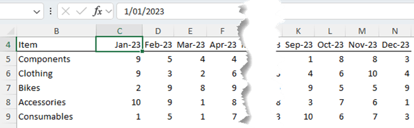
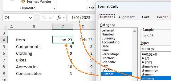
Note: the dates in row 4 are date serial numbers formatted to only show mmm-yy, as you can see in the formula bar:
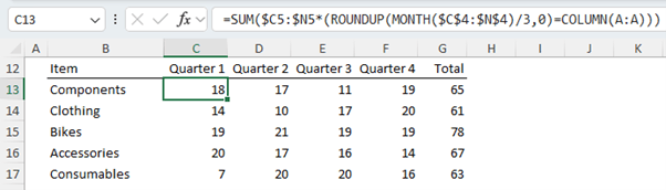
We can sum the data into quarters using the following formula in the top left cell of the table
=SUM($C5:$N5*(ROUNDUP(MONTH($C$4:$N$4)/3,0)=COLUMN(A:A)))
Which can then be copied across for the remaining quarters, and down for the other items returning a table of values summarized by quarter:
Each argument in the formula explained
=SUM($C5:$N5*(ROUNDUP(MONTH($C$4:$N$4)/3,0)=COLUMN(A:A)))
The range referenced by SUM is simply the range we want to sum by quarters.
The absolute referencing on the columns enables the formula to be copied down and across while remaining on the correct columns:
=SUM($C5:$N5
Taking row 5, it evaluates to an array of the following values
{9,5,4,4,9,4,2,8,1,8,8,3}
Next, the MONTH function returns the month number of each date in row 4.
ROUNDUP(MONTH($C$4:$N$4)/3,0)
Dividing the result by 3 and rounding it to zero decimal places results in an array of the quarter numbers
{1,1,1,2,2,2,3,3,3,4,4,4}
We use the COLUMN function to return the quarter numbers one by one
COLUMN(A:A)
The first formula references A:A, returning 1. When the formula is copied across the columns, the range referenced by COLUMN updates to reference B:B, returning 2 and so on.
When ROUNDUP(MONTH($C$4:$N$4)/3,0) = COLUMN(A:A) is evaluated it looks like this:
{1,1,1,2,2,2,3,3,3,4,4,4} = 1
And we get an array of TRUE and FALSE values:
{TRUE,TRUE,TRUE,FALSE,FALSE,FALSE,FALSE,FALSE,FALSE,FALSE,FALSE,FALSE}
When we multiply these by the array returned by the first range, $C5:$N5, the TRUE and FALSE evaluate to their numeric equivalents of 1 and 0. So we have this:
=SUM( {9,5,4,4,9,4,2,8,1,8,8,3} * {1,1,1,0,0,0,0,0,0,0,0,0} )
Which evaluates to:
=SUM( {9,5,4,0,0,0,0,0,0,0,0,0} )
=18
Tip: we can improve this formula with the LET function which enables you to name variables inside the formula, making it easier to write and make sense of when you come back to it in a few months’ time:
=LET(

    quantity, $C5:$N5,

    mths, $C$4:$N$4,

    qtrs, ROUNDUP(MONTH(mths) / 3, 0),

    currentQtr, COLUMN(A:A),

    SUM(quantity * (qtrs = currentQtr))

)
Download the example file above for the equivalent formula for data in a vertical layout.
Summarize Data into Quarters using Dynamic Arrays
With the introduction of dynamic array functions in Excel, we* can now write a single formula for each row/item in the table using the BYCOL and LAMBDA functions.
*BYCOL and LAMBDA are currently only available to users with a Microsoft 365 subscription. If that’s not you, try the PivotTable Grouping method here.
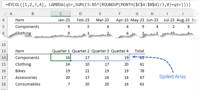
We leverage the same ROUND(MONTH(… formula component to convert the dates to their equivalent quarters and nest it in the BYCOL and LAMBDA functions like so
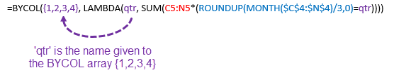
=BYCOL({1,2,3,4}, LAMBDA(qtr, SUM(C5:N5*(ROUNDUP(MONTH($C$4:$N$4)/3,0)=qtr))))
The result is a spilled array for each row, as you can see in row 14 of the image below
Each argument in the formula explained:
=BYCOL({1,2,3,4}, LAMBDA(qtr, SUM(C5:N5*(ROUNDUP(MONTH($C$4:$N$4)/3,0)=qtr))))
BYCOL returns the values of an array/range, one column at a time and provides them to the LAMBDA function, which then aggregates them.
The BYCOL function syntax is
BYCOL(array, lambda(column))
And in this example, we’re using a LAMBDA function with SUM like so
BYCOL(quarters, LAMBDA(quarters name, SUM(columns that match the quarters, one quarter at a time)))
The first argument for BYCOL is the array of quarter numbers
=BYCOL({1,2,3,4}
IMPORTANT: the comma separator between each number in the BYCOL array indicates a new column of data. A semi-colon here would indicate a new row of data.
The first argument for LAMBDA is simply the name I’ve given to the quarter numbers array in the first argument of BYCOL i.e. ‘qtr’
The range referenced by SUM is the range we want to sum by quarters
SUM(C5:N5
Taking row 5, it evaluates to an array of the following values
{9,5,4,4,9,4,2,8,1,8,8,3}
Next, the MONTH function returns the month number of each date in row 4.
ROUNDUP(MONTH($C$4:$N$4)/3,0)
Dividing the result by 3 and rounding it to zero decimal places results in an array of the quarter numbers
{1,1,1,2,2,2,3,3,3,4,4,4}
Remember, the comma separator between each value in the array indicates a new column. We then use the qtr array, one column at a time to return an array of values for SUM to aggregate.
For example, the first column of qtr is applied like so
SUM( {9,5,4,4,9,4,2,8,1,8,8,3} * ( {1,1,1,2,2,2,3,3,3,4,4,4}=1 ) )
Returning
SUM( {9,5,4,4,9,4,2,8,1,8,8,3} * {TRUE,TRUE,TRUE,FALSE,FALSE,FALSE,FALSE,FALSE,FALSE,FALSE,FALSE,FALSE} )
And when TRUE and FALSE values have a math operation applied to them, in this case multiply, they convert to their numeric equivalents of 1 and 0 returning this
SUM( {9,5,4,4,9,4,2,8,1,8,8,3} * {1,1,1,0,0,0,0,0,0,0,0,0} )
Which evaluates to
SUM( {9,5,4,0,0,0,0,0,0,0,0,0} )
=18
This value is returned to the first cell in the spilled array.
BYCOL then gives SUM the next quarter and the process starts again
SUM( {9,5,4,4,9,4,2,8,1,8,8,3} * ( {1,1,1,2,2,2,3,3,3,4,4,4}=2 ) )
Which evaluates like so
SUM( {9,5,4,4,9,4,2,8,1,8,8,3} * ( {0,0,0,1,1,1,0,0,0,0,0,0}) )
SUM( {0,0,0,4,9,4,0,0,0,0,0,0} )
=17
This value is returned to the second cell in the spilled array.
Tip: And again with the LET function so it’s easier to write and make sense of when you come back to it in a few months’ time
=LET(

    qtrArray, {1, 2, 3, 4},

    qtrs, ROUNDUP(MONTH($C$4:$N$4) / 3, 0),

    quantity, C5:N5,

    BYCOL(

        qtrArray

        LAMBDA(qtrArray,SUM (data * (quantity = qtrArray)))

    )

)
Download the example file above for the equivalent formula for data in a vertical layout.
Single Formula to Sum Data into Quarters and Categories
The previous formula is ok, but I still have to copy it down the rows.
It would be better if it automatically spilled the row and column results, so I don’t have to copy and paste at all!
However, I’d reached the limit of my current formula writing skills.
So, I reached out to the most incredible formula writers I know: Sergei Baklan and Peter Bartholomew to see if they were up for the challenge. Of course, they were.
In fact, they were so up for it they provided me with a total of 8 different formulas.
Plus, Sergei provided Power Query, Office Scripts and Python in Excel options, which you can see in the files available to download from the link above!
Rather than looking at all their solutions, we’ll just look at a few, because they each offer something different.
Note: These solutions require dynamic array functions BYCOL or BYROW, which are currently only available with a Microsoft 365 license.
Horizontal Layout Solution by Peter Bartholomew
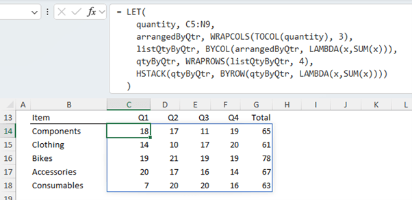
Using the data table from my previous examples, Peter’s final offering is this very succinct formula:
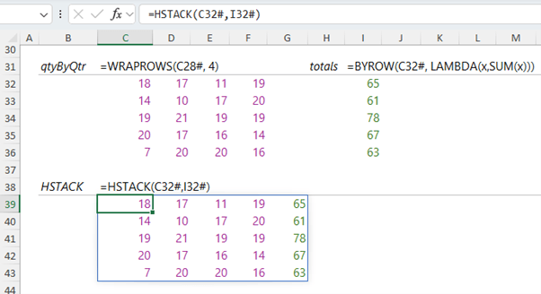
=LET(

    arrangedByQtr, WRAPCOLS(TOCOL(quantity), 3),

    listQtyByQtr, BYCOL(arrangedByQtr, LAMBDA(x, SUM(x))),

    qtyByQtr, WRAPROWS(listQtyByQtr, 4),

    HSTACK(qtyByQtr, BYROW(qtyByQtr, LAMBDA(x, SUM(x))))

)
Which returns the spilled array in cells C14:G18 shown below
Each argument in the formula explained
This formula processes the values in the table, unpivots them, groups them into quarters, and sums them up for each quarter. Then presents the quarterly sums along with an annual total.
1. Unpivot and Group by Quarters (arrangedByQtr):
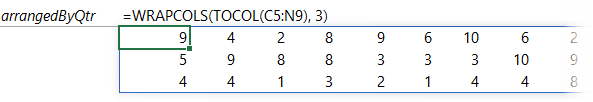
- TOCOL(quantity): This converts the 'quantity' (which is the name for the range C5:N9) into a single column.
- WRAPCOLS(TOCOL(quantity), 3): This then wraps (or reshapes) this single column into multiple columns, each having 3 rows. i.e. it rearranges the data into quarters, where each quarter has 3 months. The result is stored in 'arrangedByQtr', as shown below

2. Sum Each Quarter (listQtyByQtr):
- BYCOL(arrangedByQtr, LAMBDA(x, SUM(x))): This applies the SUM to each column of 'arrangedByQtr'. This will produce a list where each item is the sum of a quarter, stored in 'listQtyByQtr', as shown below:

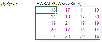
3. Arrange Quarterly Sums into Rows (qtyByQtr):
- WRAPROWS(listQtyByQtr, 4): This reshapes 'listQtyByQtr' into multiple rows, with each row having 4 values. i.e. the data across years, where each year has 4 quarters. The result is stored in 'qtyByQtr', as shown below:
4. Add Row-wise Total:
- HSTACK(qtyByQtr, BYROW(qtyByQtr, LAMBDA(x, SUM(x)))): This horizontally stacks the 'qtyByQtr' array with the row-wise sums of 'qtyByQtr'. The 'BYROW(qtyByQtr, LAMBDA(x, SUM(x)))' function calculates the sum for each row in 'qtyByQtr'.
The overall output of the formula is an array where each row represents the summed quantities for each year (broken down by quarters), followed by a total quantity for that year.
Horizontal Layout Solution by Sergei Baklan
The image below displays the result of a single formula in cell B13 that spills the results for the entire table, including column and row labels:
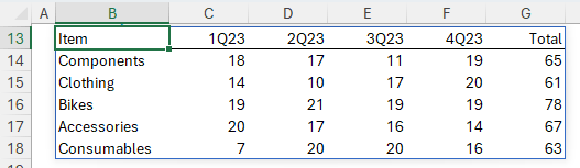
It’s constructed using this single formula based on the horizontal layout used in the examples above
=LET(

    data, DROP(range, 1, 1),

    total, BYROW(data, LAMBDA(v, SUM(v))),

    months, DROP(TAKE(range, 1), , 1),

    MonthsInQuarters, ROUNDUP(MONTH(months) / 3, 0) & "Q" & RIGHT(YEAR(months), 2),

    quarters, UNIQUE(MonthsInQuarters, 1),

    nRows, ROWS(data),

    nCols, COLUMNS(quarters),

    sums, MAKEARRAY(

        nRows,

        nCols,

        LAMBDA(n, m,

          INDEX(

            BYROW(

              data,

                LAMBDA(v,

                  INDEX(

                     MMULT(v, --(TRANSPOSE(MonthsInQuarters) = quarters)), 1, m))

                ), n,1)

        )),

    HSTACK(

      TAKE(range, , 1),

      VSTACK(quarters, sums),

      VSTACK("Total", total)

    )

)
Each argument in the formula explained:
This formula processes a table of data with monthly columns, aggregates the data into quarterly columns, and appends a total for each row at the end. It can be explained as follows
1. Initialize Data:
- data, DROP(range, 1, 1): Removes the first row and first column from the 'range'. This gets the data excluding the header row.
- total, BYROW(data, LAMBDA(v, SUM(v))): Calculates the sum of each row in the 'data'.
- months, DROP( TAKE(range,1),,1): Takes the first row of the 'range' (which contains dates) and drops the first column.
2. Convert Months to Quarters:
- MonthsInQuarters, ROUNDUP(MONTH(months)/3,0) & "Q" & RIGHT(YEAR(months),2): Converts each month in 'months' to its respective quarter representation, e.g., "1Q23" for January 2023.
- quarters, UNIQUE(MonthsInQuarters,1): Extracts the unique quarters from the 'MonthsInQuarters' array.
3. Determine Dimensions:
- nRows, ROWS(data): Counts the number of rows in 'data'.
- nCols, COLUMNS(quarters): Counts the number of unique quarters.
4. Calculate Quarterly Sums:
- sums, MAKEARRAY(...): Creates an array of size 'nRows x nCols' where each element represents the sum of values for a specific quarter.
- The inner 'MMULT' function multiplies each row's values with a matrix indicating which month belongs to which quarter. The result of this multiplication gives the quarterly sum for each row.
5. Combine Results:
- HSTACK(...): Horizontally stacks the following:
- The first column of the original 'range' (The column labels).
- A vertically stacked array consisting of the unique 'quarters' followed by the 'sums'.
- A vertically stacked array consisting of the label "Total" followed by the row totals ('total').
The final output is a table where the data is aggregated on a quarterly basis, with the last column showing the total for each row.
Sergei also offered two more formula options, one using a thunk and another using MAKEARRAY.
They can be downloaded from the workbook download link above.
Vertical Layout by Peter Bartholomew
The final challenge I only put to Peter was, what if we needed to allow for more than 12 months and a variable number of categories using the vertical data layout shown below:
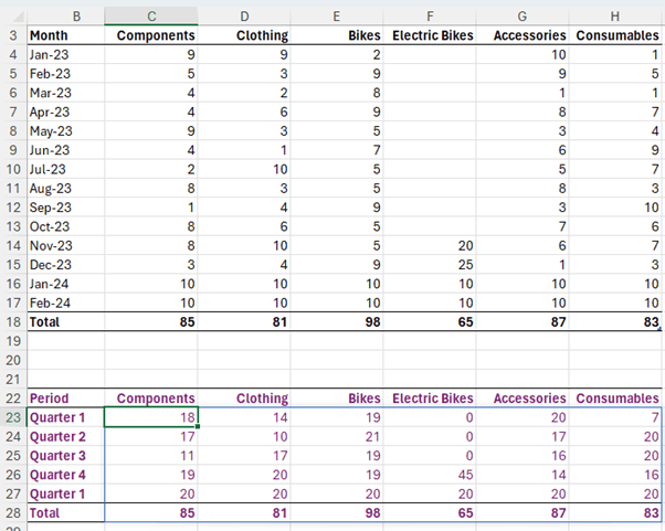
This is Peter's solution.
=LET(

    m, 1 + QUOTIENT(ROWS(quantityV) - 1, 3),

    expanded, EXPAND(quantityV, 3 * m, , 0),

    arrangedByQtr, WRAPROWS(TOCOL(expanded, , TRUE), 3),

    listQtyByQtr, BYROW(arrangedByQtr, SUMλ),

    qtyByItem, WRAPCOLS(listQtyByQtr, m),

    qtyByItem

)
Each argument in the formula explained:
The formula uses the 'LET' function, which allows for the creation of named intermediate variables within a formula, helping to break down complex calculations.
1. Calculate the Number of Columns:
- m, 1 + QUOTIENT(ROWS(quantityV) - 1, 3): The 'QUOTIENT' function divides the number of rows in 'quantityV' minus one by 3 and returns the integer portion of the division. Adding 1 to this result gives 'm', which represents the number of columns required when the data is grouped in sets of 3 rows.
2. Expand the Data:
- expanded, EXPAND(quantityV, 3 * m, , 0): The 'EXPAND' function likely enlarges the range of 'quantityV' to have (3 * m) rows. Any new cells created by this expansion are filled with zeros.
3. Convert to Single Column and Group by Threes:
- arrangedByQtr, WRAPROWS(TOCOL(expanded,,TRUE), 3): 'TOCOL(expanded,,TRUE)' converts the 'expanded' range into a single column, ignoring any empty cells.
- WRAPROWS(..., 3) then takes this single column and wraps it into multiple rows, with each row having 3 values. This is effectively grouping the values in sets of three.
4. Sum Each Group:
- listQtyByQtr, BYROW(arrangedByQtr, SUMλ): For each row (which has 3 values) in 'arrangedByQtr', the sum of those values is calculated using 'SUMλ'. The result is a single column where each row represents the sum of a group of three values from the original data.
5. Organize Sums by Item:
- qtyByItem, WRAPCOLS(listQtyByQtr, m): This takes the single column of sums ('listQtyByQtr') and wraps it into multiple columns, each having 'm' rows. If 'quantityV' had rows representing different items and columns representing different time periods (e.g., months), then 'qtyByItem' would have rows representing items and columns representing quarters.
6. Output the Result:
- The final output of the formula is 'qtyByItem', which is an array where each row represents a quarter, and each column represents the sum of quantities over categories.
In summary, this formula aggregates data from 'quantityV' over groups of three (i.e., summing monthly data into quarters) and then presents these aggregated sums in a table where each row represents a quarter, and each column represents a category.
Too Hard? Use a PivotTable
If all those formulas are hurting your head, there is an easier way using a PivotTable grouping.


What a relief to find a link at the very end, to do it with pivot tables 🙂
Nevertheless epic work ! Thanks for sharing !
I like the solutions with powerquery too – love that tool.
thanks for sticking with it to the end, Danny. I love and prefer the Power Query & PivotTable solution too!
Hi, I enjoyed the video, not really falmiliar with most of these new functions, but it seems to me that this would work using an old function:
=LET(
quantity,$C5:$N9,
mths,$C$4:$N$4,
qtrs,ROUNDUP(MONTH(mths)/3,0),
MMULT(quantity,TRANSPOSE(N(qtrs=SEQUENCE(5))+N(SEQUENCE(5)=5))))
Very nice, James! You’re now the 3rd person I know that is awesome at writing formulas
Your introduction only mentions the 2 formula methods.
Then at the very end you mention pivot tables.
Please edit the introduction to mention the Pivot tables. Maybe even mention using PowerQuery to UnPivot raw data if it is in the wrong format.
While formulas are the “traditional” method, as you know, PivotTables are so much easier and faster, especially when you want to modify them.
Hi Ron,
Thanks for reading the post. The table of contents at the beginning mentions the PivotTable option. Not everyone wants to use a PivotTable for this, which is why I’ve done this post on the formula solution and a separate post on the PivotTable method.
Mynda
Sorry, from my earlier the post, the dates should be fully absolute, so:
This is what I have been using, I think it is a little easier to understand off the bat, but I may be wrong and it just makes more sense to me!
=SUM(–(CHOOSE(MONTH($C$4:$N$4),1,1,1,2,2,2,3,3,3,4,4,4)=COLUMN(A:A))*$C5:$N5)
Also, it has the added advantage that if your quarters aren’t standard (eg my FY starts in Aug, so my first quarter is Aug-Oct) then simply adjust the numbers in the quarters’ array to fit, so, for my Aug starting FY:
=SUM(–(CHOOSE(MONTH($C$4:$N$4),2,3,3,3,4,4,4,1,1,1,2,2)=COLUMN(A:A))*$C5:$N5)
Nice, Duncan. Thanks for sharing. I’ve used the CHOOSE method for fiscal periods too, but hadn’t considered it for calendar quarters.
awesome amazing , i was struggling to find a solution of converting Monthly data to Quarterly and you make my life easy
what is the criterion to decide 3 in row function formulae ie 3*row()-3
Glad it was helpful, Sahil! I’m not sure what you mean by ‘decide 3 in row’. Please post your question and sample Excel file on our forum where we can help you further: https://www.myonlinetraininghub.com/excel-forum
Firstly the Summarise Monthly Data into Quarters – Horizontal Data instructions are awesome and worked perfectly, thank you so much.
I have a question, for my data set I have set up quarter columns for two years worth of data. I generate a monthly report so sometimes there isn’t data for all three months in the quarter. Is there a way to set up an additional column or even a cell that will identify what quarters only have partial months data and what months have data?
Thank you
Hi Melanie, I’m glad you found the formula helpful. Yes, you can detect if a period doesn’t have 3 months of data in a quarter. The formula will depend on how your data is laid out and what you hope to then do with that information. Please post your question and sample Excel file with an example of the result you want on our forum and we can help you further.
Mynda
This is interesting. Suppose if I don’t want to use Sum function and I just want to extract the value from the row, how can one use this formula? Just one thing to note, the value that needs to be extracted is from time cards, so in some cases there will be five rows for Monday-Friday and in some Monday to Thursday or whatever days they worked. Long story short the values that need to be extracted are not at regular intervals i.e. every 5 lines or 4 lines.
Hi Mithil,
Please post your question and sample Excel file containing a before and after example on our Excel Forum so we can help you further.
Mynda
i have an excel where the months are Dec 2019 thru Feb 2020. How do I make sure my formula totals this as two quarters?
Hi Geetha,
I’d use a PivotTable and the build in grouping tools.
Mynda
Great solution and explanation, thanks so much
You’re welcome.
These formula look useful but I can’t get it to work in my case. I need to aggregate monthly data in to quarters. I also need the formula to understand that quarters are Jan-Mar, Apr-June, Jul-Sep, and Oct-Dec.
My data is laid out like this:
Months (B1:P1) – Cell P1 references user input for reporting month from a different sheet.
Data (B3:P133) – each row has a different indicator)
I tried =SUM(OFFSET($B2,,3*COLUMNS($B$2:B2)-3,1,3)) but it of course does not care about the month data.
I also tried to use Catalin’s formula =SUM(OFFSET($A$2:$C$2,0,MONTH(DATEVALUE(“01 “&Sheet1!A1&” 2017″))-1)) but was unable to produce the result I am looking for. Any ideas?
I can easily get the formulas to add three consecutive months but that doesn’t account for the shift in months based on the referenced month and then they are no longer quarters. This report is updated every month.
Hi Jonathan,
Can you please open a new topic on our forum? You can upload a sample file so we can see and work on your exact structure.
Cheers,
Catalin
I just wanted to say that I found this really helpful. Thank you!
Glad we could help, Tris 🙂
i want to know how to calculate my monthly purchases, from an yearly purchase sheet, when there are many purchases in a single month. please help.
Hi Mangal,
You will have to provide an example of your data, use our forum to upload a sample file. (create a new topic after sign-up). There can be too many solutions, depending on your data structure.
Catalin
How do I use the sum offset formula to add any 3 months of the year depending on the month I pick from the drop down menu which is in another tab?
Thanks.
Hi Ricky,
This formula:
=SUM(OFFSET($A$2:$C$2,0,MONTH(DATEVALUE(“01 “&Sheet1!A1&” 2017″))-1))
will offset the range A2:C2 depending on your selection from Sheet1!a1 (assuming that is the dropdown cell). If you select January, the range will be the same as the initial range, first 3 columns (MONTH number-1 will be 0). If February is selected, the range to sum will be offset by 1 column , Feb-Mar-April data will be added. Same result can be obtained with another similar formula:
=SUM(OFFSET($A$2:$C$2,0,INDEX({0,1,2,3,4,5,6,7,8,9,10,11},MATCH(Sheet1!A1,{“January”;”February”;”March”;”April”;”May”;”June”;”July”;”August”;”September”;”October”;”November”;”December”},0))))
Note that if november or december is selected, there should not be 3 cells to add, only 2 or 1. In this case, you should use the “Width” argument of the OFFSET function to shrink the initial range to 2 or 1 column.
Thank you. Let me try that. This should work for months going across columns right? I’m adding the PREVIOUS 3 months so November and December should not be a problem. I start with March as the first month in Source from data validation table.
Thanks.
Yes, months should be in columns. If you need more help on this subject, a sample file will help us understand your exact situation. You can upload it on our forum (create a new topic after sign-up)
Thank you so much! Your help is really appreciated.
I love your formula thank you it is saving me so much time
Thanks, Rana. Glad I could help.
Mynda
=SUM(OFFSET($L2,,3*COLUMNS($L$2:L2)-3,1,3))
Hi great stuff, but I guess I’m one of those ‘one percenters’ who need a little extra help…
Your ‘in plain English’ explanation of the vertical formula was great I ‘almost’ got it.
BUT no ‘plain English’ for the horizontal which is the one I actually need!!!!
So ok
SUM – yes I get it – summing something
OFFSET – yup – moving ranges of the formula to the appropriate range
(I’m creating quarterly data from monthly data, monthly on one tab and quarterly on another)
$L2 – don’t quite understand the ‘absolute reference’ to the column since columns changing across quarters. I DO get that this is the ‘reference’ cell. guess the formula always needs to have the ‘reference cell’ in it?
,, – Do not understand why there are two comma marks?
3*COLUMNS – not sure what that means. Does that mean there are 3 columns? and why multiplied?
$L$2:L2 – really lost on exactly what this means, maybe again must have the ‘reference cell’ which is the beginning of whatever the formula is and wherever it goes on the spreadsheet, starting point always there
-3,1,3 – have no idea what the negative 3 means in this formula. assuming 1 is one row high and 3 is 3 columns wide??
THANK YOU!
Hi Michael,
The 3*COLUMNS(…)-3 is because there are 3 months in a quarter, so you want to jump 3 columns across at a time and include 3 columns in your SUM range. The COLUMNS function returns the count of columns in the range specified.
The $L$2:L2 uses absolute referencing on the first cell reference and not the second so that when you copy the formula to other cells the L2 updates accordingly. e.g. L2 will become M2 and so on as you copy it across the columns.
The first argument of OFFSET, $L2 is the starting point/reference argument for the OFFSET function.
The two consecutive commas are placeholders for the arguments in OFFSET that we don’t need to use. More on how OFFSET works here.
To get a better understanding I recommend you download the workbook and use the Evaluate Formula tool to see how the formulas are evaluating. Try it on cell L9 and then look at cell M9 and M10 to see the differences.
Mynda
Both are quite useful examples,, plz post more on Data analysis.
Wow!
It saved me huge amount of monkey job time )
Thank you!
Great help – thank you!! My heart sank when I found another vertical example so very pleased to scroll down and find a horizontal example too.
Glad we could help, GD 🙂
This is great, thanks very much!
Question: what if their are multiple rows with the same month and I want to aggregate them by quarter as well.
For example in your file there would be three of each month and I still want them to be in quarter file.
Does this still work?
Thanks
Raeann
Hi Raeann,
To be honest, I’d use a PivotTable. Just make sure you have a column that contains proper dates, then you can use the Group tool in the PivotTable to automatically summarise them into quarters:
https://www.myonlinetraininghub.com/excel-pivottable-group-data-video
Mynda
Wow, I don’t have words to describe this tutorial, everything I can say is little compared to its power. Excellent, Mynda, you are always pushing the boundaries of Excel!!
🙂 Wow, thanks Juan. Glad you found it useful.
Mynda
This formula is truly amazing and impressive, it really shows the power of Excel knowledge, what a great strategic use of functions! Yesterday I sent the workbook example to some co-workers and they were totally impressed with what can be achieved!!
🙂 nice!
I like to use the =if(mod(month(cellref),3)=0,sum(cellref:offset(cellref,x,x)),0) function in a rolling dataset and use index/match to pull the data needed in a summary table matching the date reference. You can replace the 3 in the mod function with a 6, 9, 12 to get x months ending totals as well as long as you make sure the offset variable matches the mod variable (3 in this case).
Nice tip. Cheers, Kevin 🙂
which can be read as “if the category at entry C42 to C2000 equals the one at A4…” The $ signs make the formula use absolute references so that when I duplicate the formula, it won’t shift the references. 42 refers to the first row where ledger entries begin. 2000 is an arbitrary large number I am not likely to reach. You can think of $C$42:$C$2000 as being equivalent to something like “C:C” from the first examples. A4 is a reference to a specific category name from the top section.
Hi Louisa,
I don’t quite get your problem here.
Please do clarify if there’s anything
you need. You may also send some file
here: HELP DESK.
Cheers,
CarloE
The formula above returns the count for the entire range of dates but I need to find the number for each month, ie the number for May, June etc. How would that be done?
Hi Stephanie,
I’m not sure I understand your question since the numbers for each month are already summarized in this example. If you have multiple instances of dates for each month that you want to sumamrize there are a few options:
1. SUMIFS
2. SUMPRODUCT
3. PivotTables
I hope that helps.
Kind regards,
Mynda.
Hi Mynda,
I hope you’ll post here my suggestion for a more “realistic” situation in which there is more than one instance per month [using the SUMPRODUCT function].
BTW, I don’t think that this can be solved with the SUMIFS function, but of course I might be wrong….
Best Regards,
Meni Porat
Hi Meni,
Thanks for your suggestion. My example is taking data that has already been summarised into a monthly report, but you could summarise the source data into quarters using SUMPRODUCT or SUMIFS.
SUMIFS allows multiple criteria (in this case start and end dates for each quarter), just as SUMPRODUCT does.
As with most things, Excel had many ways to ‘skin a cat’ 🙂
Kind regards,
Mynda.
This was a very informative one for me.
Thank you very much.
Thanks, Babu. Glad you liked it 🙂
Thanks Minda,
Very good tutorial. Actually I was looking for the same trick..
Thanks Again..
Thanks, Vishal 🙂 Glad I could help.
I would group this data using a pivot table. Group the months into Quarters. I do use the OFFSET function frequently – but a pivot table seems easier in this instance
Hi Yvonne,
Yes, but that would spoil the formula fun 🙂
Cheers,
Mynda.