If you’re familiar with array formulas, then the simplicity of Excel Dynamic Arrays will be a breath of fresh air. And if you’ve always shied away from array formulas then Dynamic Arrays are for you.
Excel no longer requires you to enter array formulas with CTRL+SHIFT+ENTER and formulas that return multiple results will now automatically ‘spill’ into the cells below and or to the right, as you can see below:
Before Dynamic Arrays the ROW formula above would return 1 because it can only display the first value in a single cell, but now that it can ‘spill’ into the cells below, it returns the values 1 through 4.
Previously we would have to select cells A1:A4 prior to entering the ROW formula and then press CTRL+SHIFT+ENTER to return the array. I think you’ll agree it’s now far simpler.
Also notice in the formula bar above that there aren’t any curly braces around the formula to indicate it’s an array formula. And when I move my cell selection away from A1 you can see the formula bar now contains a ghosted formula, indicating I can’t modify it.
This new ‘spill’ result gives Excel array functions transparency and makes them more easily discoverable, getting users up and running with array formulas more quickly than ever before.
Array formulas are no longer limited to super users, they are for everyone!
Note: Dynamic Arrays are only available in Excel 2021 onward or with a Microsoft 365 license.
Table of Contents
Download the WorkbookUNIQUE Function
SORT Function
Dynamic Arrays with Data Validation
FILTER Function
Dynamic Array Effect on Existing Functions
Implicit Intersection
Backward Compatibility
#SPILL! Errors
Dynamic Array Limitations
More Excel Dynamic Arrays
Download the Workbook & Cheat Sheet
Enter your email address below to download the files.
 Download the Cheat Sheet.
Download the Excel Workbook. Note: This is a .xlsx file please ensure your browser doesn't change the file extension on download.
Let’s look at some of the cool new functions.
UNIQUE Function
Extracting unique or distinct values from a list is a common requirement and up until now you could either use a complicated array formula like this:
=IFERROR(INDEX($C$7:$C$21,MATCH(0,COUNTIF($B$26:B26,$C$7:$C$21),0)),"")
Or we could use a PivotTable or Power Query to extract a unique list.
However, now that we have the UNIQUE function the formula above can be replaced with this:
=UNIQUE(C7:C21)
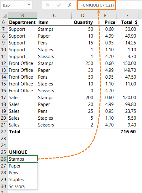
You’ve got to admit, it doesn’t get much easier than that!
The syntax for the UNIQUE function is:
=UNIQUE(array, [by_col], [occurs_once])
array is the range or array you want the unique values returned from.
by_col is an optional logical value (TRUE/FALSE) and allows you to compare values by row (FALSE), or by column (TRUE). You can see in the example above that I omitted it, which means it will default to FALSE and sort by row.
occurs_once is also an optional logical value (TRUE/FALSE) and allows you to find the truly unique values, i.e. the values that only occur once (TRUE), or all distinct values (FALSE). If you omit this argument, as I have done above, it will default to FALSE and return a distinct list.
SORT Function
It’s nice to be able to easily get a distinct list with the UNIQUE function, but what if you also want it sorted. The old array formula approach was something scary like this:
=IFERROR(INDEX($A$26:$A$30, MATCH(SMALL(IF(COUNTIF($B$26:B5, $ A$26:$A$30)=0, COUNTIF($A$26:$A$30, "<"&$ A$26:$A$30), ""), 1), COUNTIF($A$26:$A$30, "<"&$ A$26:$A$30), 0)),"")
But you’ll be pleased to know there’s a new SORT function that you can simply wrap around UNIQUE like so:
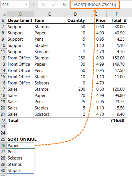
The example above is SORT in its simplest form, but the syntax for the SORT function has some more optional arguments:
=SORT(array, [sort_index], [sort_order], [by_col])
array is the range or array containing the values you want sorted.
sort_index is optional and indicates the row or column to sort by. When omitted it will default to sort by the first row or column in the array.
sort_order is optional. It’s a number; 1 for ascending and -1 for descending. If omitted, it will sort in ascending order.
by_col is an optional logical value (TRUE/FALSE) indicating the desired sort direction; FALSE to sort by row (default), TRUE to sort by column. You can see in the example above that I omitted it, which means it will default to FALSE and sort by row.
Data Validation
Now that we have our nicely sorted unique list it makes sense that you might want to use it in a data validation list. To reference a spilled array we simply use the new Spilled Range Operator, #, as shown in the Data Validation ‘Source’ field below:
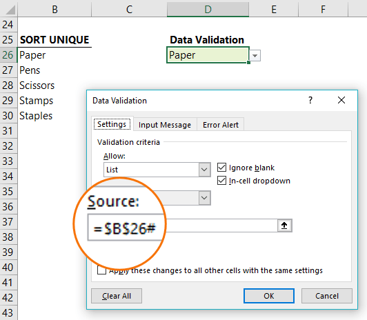
When we reference the spilled range using the # notation it will automatically adjust to include new cells as the spilled range grows, or exclude rows as the range contracts. In other words, it’s a dynamic reference. And I haven’t had to go near OFFSET or INDEX to create it!
Tip: The Spilled Range Operator gets automatically inserted if you select the whole spilled range of cells in a formula e.g.
=COUNTA(B26:B30) would be converted to =COUNTA(B26#) as you can see below:
Unfortunately, it doesn’t automatically insert the spilled range operator in the Data Validation List source field…yet.
FILTER Function
The FILTER function returns a range filtered on criteria you define. In the example below, we have returned the records from the table in cells B7:F21 for ‘Stamps’, as selected in the data validation list in cell B25.
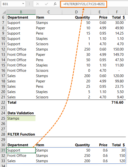
Notice the spill range is cells B31:F33 as denoted by the blue border around the cells.
In English the formula in cell B31; =FILTER(B7:F21,C7:C21=B25), reads:
Return the records from the table in cells B7:F21, where the values in cells C7:C21 = the value in cell B25, which is ‘Stamps’.
The syntax for FILTER is:
=FILTER(array, include, [if_empty])
array is the range or array containing the values you want to filter.
include is the logical test instructing FILTER which rows to include in the filtered result. It returns an array of Boolean values (TRUE/FALSE).
If_empty is optional. It’s the value to return if all values in the included array are empty.
Tip: We can filter by multiple criteria by adding logical tests e.g.
Filter for Stamps AND Support:
=FILTER(B7:F21,(C7:C21="Stamps")*(B7:B21="Support"))
Filter for Stamps OR Paper
=FILTER(B7:F21,(C7:C21="Stamps")+(C7:C21="Paper"))
Dynamic Array Effect on Existing Functions
As I mentioned at the beginning, Dynamic Arrays have changed the way the Excel calc engine treats functions that can return a range, in that they can now spill. It also means that some functions that didn’t previously return arrays can also spill if you reference a range in an argument that is expecting a single value/cell (scalar).
For example, the COUNTIF formula below spills because the criteria argument is given the spilled range i.e. =COUNTIF(C7:C21, $B$25#)
Implicit Intersection
Warning, the following content is advanced, and you don’t need to know it or understand it, so read on if you wish.
If you’re familiar with implicit intersection then you may be thinking that the COUNTIF formula above is relying on implicit intersection to return the correct count, but with dynamic arrays it’s not. You could move the COUNTIF formula anywhere in the worksheet and it would still return the spilled array, as you can see below where COUNTIF is now offset by 1 row to the list of count criteria:
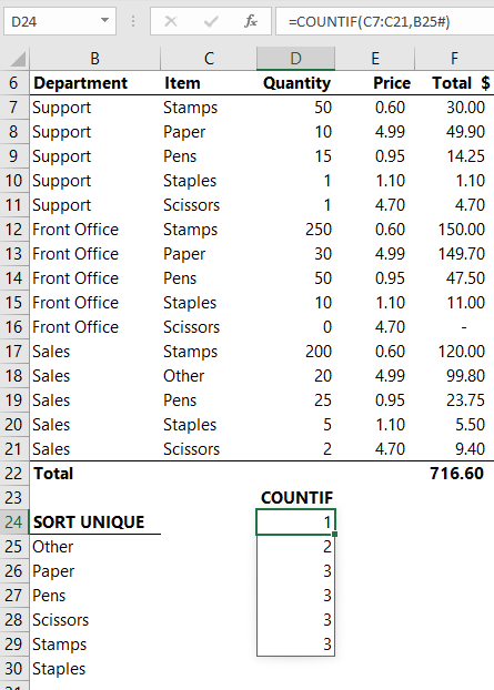
In older versions of Excel this would break the COUNTIF formula.
In fact, this is one of the fundamental changes to the Excel calc engine. Implicit intersection is no longer the default. Instead if you want a formula to evaluate implicitly you need to prefix the range or formula that returns the range with the @ symbol.
For example, the COUNTIF formula example given earlier; =COUNTIF(C7:C21,$B$25#), would become:
=COUNTIF($C$7:$C$21,@$B$25#)
Backward Compatibility
If a user opens a workbook containing a dynamic array Excel will automatically convert it to a legacy array formula surrounded by curly braces. When you open it again in Office 365 it will remove the curly braces.
If you use one of the new array functions, or use the Spilled Range Operator (#), it will prefix it with _xlfn to indicate that the function is not supported in the version of Excel you are currently in. You can see an example of this in the Excel 2013 screenshot below:
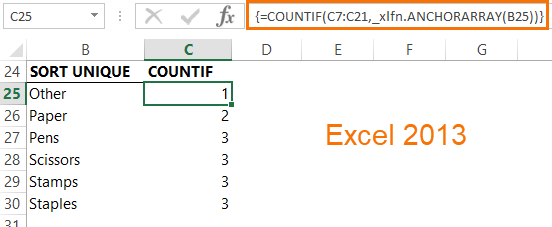
As long as you don’t edit the formula Excel will display the results and you can reference these cells in other formulas etc. If you edit the formula it will break.
#SPILL! Errors - Range Isn’t Empty
If you have data in the path of a Spill you’ll get the #SPILL! Error like so:
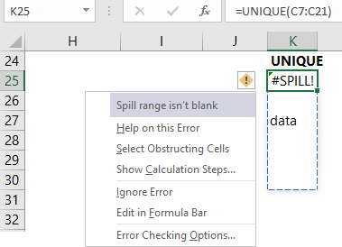
Clicking on the warning icon will reveal a list of options for rectifying the problem. Or you can just delete the problem data and it will Spill.
Dynamic Array Limitations
There is limited support for references between workbooks. Dynamic Arrays require both workbooks to be open, otherwise you will get #REF! errors.
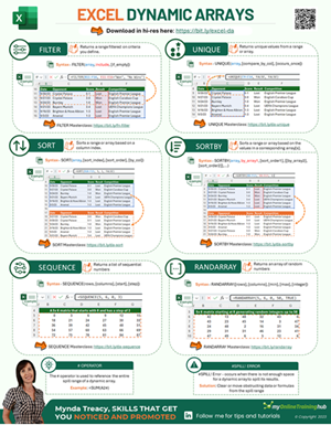
More Excel Dynamic Arrays
This is just the beginning and a taste of some of the Dynamic Array functions. Check out our comprehensive tutorials on some of the other new Dynamic Array functions:
| FILTER | Filter cells based on criteria. |
| RANDARRAY | Returns an array of random numbers between 0 and 1. |
| SEQUENCE | Returns list of sequential numbers that increment as specified. |
| SORT | Sort cells or arrays in ascending or descending order. |
| SORTBY | Sort a range or arrays based on criteria. |
| UNIQUE | Extract a unique or distinct list from a range or array. |
Array Shaping Functions
Note: these functions are only available to Microsoft 365 users.
| EXPAND | Expands or pads an array to a specified number of rows and columns. |
| TOROW | Returns the array in a single row. Useful for combining data across multiple columns and rows into a single row. |
| TOCOL | Returns the array in a single column. Useful for combining data across multiple columns and rows into a single column. |
| WRAPROWS | Lets you wrap (reshape) a row or column of values into rows, you specify the number of values in each row. |
| WRAPCOLS | Lets you wrap (reshape) a row or column of values into columns, you specify the number of values in each column. |
| DROP | Remove a specified number of contiguous rows or columns from the start or end of an array. |
| TAKE | Extract a specified number of contiguous rows or columns from the start or end of an array. |
| CHOOSEROWS | Extract rows from the specified column or columns. |
| CHOOSECOLS | Extract columns from the specified rows or rows. |
| VSTACK | Combine arrays arranged vertically into a new single array. |
| HSTACK | Combine arrays arranged horizontally into a new single array. |
Final Word
For any Google Sheets fans out there, while you may already be familiar with the Google versions of the SORT, FILTER and UNIQUE functions, I think you'll agree the new spilled range operator (#) is going to be super useful. And the way existing Excel functions now also spill will open up a host of solutions we can't even imagine right now. Exciting times ahead!

Hi
I have a question.
Can I use Dynamic Arrays in a table? Why do I have a spill error when I use the unique function in a table?
Thanks
No, dynamic arrays are not possible in tables, sorry.
Brilliant, as usual article!
I played around with the data you provided: Created a Structured Table of the data and also two identical Data validation lists which I applied the OR functionality to.. Works brilliantly.
Also bought Bill Jelens book: Thanks for the heads up
Great to hear, Ash!
Hi, Mynda:
Thanks for an interesting article!.
I am wondering how these new dynamic functions will interface with older versions of Excel. Obviously, they won’t function as they will with Excel 365, but in particular, are there any which will break if read into older versions and then back into the Excel 365 version?
The reason I ask is that I maintain a version of Excel 2013 on one of my machines which I have purposely kept intact versus moving to 365 because it can fix some issues I have seen in Excel 365. In particular, I have been seeing occasional cases of an “Unable to find Project” error, in which the VBA project disappears and the workbook is corrupted. If I don’t save, but try to re-open the original file, the same error occurs. However, I have found that by opening the pre-corrupted version in Excel 2013 and saving it results in a recovered file I can again use in Excel 365.
However, given the extensive changes for dynamic array formulae, I’m wondering if a pass through an older version may break some of those. Any ideas?
Hi Glenn,
The dynamic array formulas won’t break if the file is opened in an older version of Excel unless the user tries to edit them, but that is the same for any function that’s not available in Excel 2013. See the “Backward Compatibility” heading in the post above which illustrates the user experience in Excel 2013.
Mynda
Thanks, Mynda. I guess it helps if you read the entire post…
hi there.
Ive checked many sites. yours is the most deep I get.
I want to filter based on a small list.
I applied same logic from countif but in FILTER function in the include part.. it doesnt work.
example:
=FILTER(Sheet2!A:X;Sheet2!C:C=B1#)
Hi Osvaldo,
FILTER cannot take a dynamic array in the ‘include’ logical test. i.e. B1# cannot be evaluated. You must enter the criteria one by one as OR criteria as explained in the FILTER Function tutorial.
I hope that helps.
Mynda
I am really excited about the capabilities of the new Excel! About eight years ago I (when I was 73) put Excel to use predicting outcomes of NY’s Lottery System. I religiously gathered and use the data for 5 years, and with truly encouraging success. The latest version of Excel has great potential, but I’m having difficulty using the Forecast formulas; thedy don’t function like the ones I’m used to. I could sent you a copy of some of that project I mentioned above. Could you possibly help me with this?
Hi Christopher, great to hear you’re enjoying Excel’s new features. Please post your questions on our Excel forum where you can share your small, sample Excel files and we can help you further. Mynda
Hi Mynda,
I’m loving Dynamic Arrays and finding new ways to exploit them all the time
What I want to do today is to repeat a value over a specified number of rows
The best I’ve come up with so far is:
=”valuetorepeat”&TEXT(SEQUENCE(noofrows,,value,0),””)
that’s OK but a little clumsy; I bet there’s a more elegant way?
NB the “valuetorepeat” is a piece of text, not a number; that’d be easy ( =SEQUENCE(value,x,,0) )
jim
Hi Jim,
Like you say, if you wanted to repeat numbers it’d be easy 🙂
You could use an IF formula e.g.where your formula is in cell B2 and you want to repeat the text 5 times:
=IF(ROWS($A$3:A3)>5,””,”TextTorRepeat”)
Copy down column.
Mynda
yes, but that’s not using the DA functionality – much more satisfying when you type formula and it magically spills down for you
Yeah, but there aren’t any DA Functions that do this…yet.
These new functions are great! However, I won’t use Office 365.
That’s a shame for you George. These new functions are incredible.
good day to all,
thank you very much again for this informative article. it help me a lot.
You’re welcome. Have fun with dynamic arrays 🙂
I have 365 Pro + Excel installed … however I tried to find a way to install this dynamic arrays but I can’t… any suggestions how to proceed further?
Thank you in advance
Hi Armin,
You can’t install dynamic arrays as such, it’s currently released to the Monthly update channel. If you’re on a semi-annual update channel, then you won’t have them yet. Speak to your IT administrator to get your update channel changed to Monthly.
Mynda
It is disappointing to hear that the dynamic arrays will not be available in Excel 2019 when it’s competitor (Google Sheets) already have them.
It is indeed, but I think it was simply a timing issue for Excel 2019 because it came out before Dynamic Arrays were released, as opposed to any kind of marketing ploy. They’re still technically in beta.
Hi Mydna,
I like your description: “If you’re familiar with array formulas, then the simplicity of the new Excel Dynamic Arrays will be a breath of fresh air.”. Can’t agree more…. 🙂
I have tried the Dynamic Arrays and they are simply awesome! The only limitation is the “user” base. When we are all excited about the new features offered in Excel 365, a majority of workplaces is still using Excel 2013… or even earlier version of Excel. Think about how you feel when you are driving a Mercedes at leisure but Honda at work… haha 😛
Here’s an article to share: create a shrinking dropdown using Dynamic Arrays.
https://wmfexcel.com/2018/11/14/dynamic-shrinking-dropdown-with-dynamic-arrays-in-excel-365/
That was the moment of my breath of fresh air. 🙂
Hope you like it.
Cheers,
MF
Hi MF,
I don’t think having users on Excel 2013 will put people off using Dynamic Arrays because Excel will convert them to regular array formulas when the file is opened in a version of Excel that doesn’t have Dynamic Arrays. Then when and Office 365 user opens the file they will be converted back to Dynamic Arrays.
Nice post on the shrinking drop down. I’m hoping the Data Validation list limitation issue will be resolved…hopefully before General Release.
Mynda
Thanks Mynda.
Indeed, many nice features in Excel 2010/2013 are still “to be discovered” to most “regular” Excel Users. I think Microsoft is doing better and better to promote new features and capabilities of modern Excel in recent years. Having said that, words of mouth from MVP like you are more powerful.
Cheers,
MF
I am using Excel 2016. The formulas shown such as UNIQUE and ARRAY does not seem to work on my excel version Is there a reason. I can’t even find the formula in the list.
Hi Danny,
Dynamic arrays are only available in Office 365 and currently only on the Insiders channel.
Mynda
FWIW, this function is not yet available on Office 365 for Mac. Looks like they’re releasing it to selected users. I have Insider Fast turned on.
There’s a note in Excel Help:
“Note: September 24, 2018: The UNIQUE function is one of several beta features, and currently only available to a portion of Office Insiders at this time. We’ll continue to optimize these features over the next several months. When they’re ready, we’ll release them to all Office Insiders, and Office 365 subscribers.”
Hi Stevek,
I’m not sure about the Mac release cycle, but hopefully it’s not too far away.
Mynda
Mynda,
Thank you for an exciting post. This sounds incredibly powerful.
I just have a question regarding operating speeds. One of the reasons that I would try to avoid array formulae was because of the massive impact it would have on operating speed. Do you know if the new dynamic version of arrays has addressed this, or will I still need to be pretty judicious in their use?
Thanks,
Hi Linda,
It’s early days still but I expect they will be more efficient. Party because you will be able to replace some of the complex array formulas with the built in functions now available. There have also been some recent changes to improve performance. You can read more about them here.
Mynda
It did not work currently using Excel 2019
Hi George,
No, Excel 2019 will never have the Dynamic Array functions, sorry. You might have missed this paragraph above:
“Note: At the time of writing Dynamic Arrays are only available in Office 365 and are currently in beta on the Insiders channel. We don’t have an ETA for when they will be available to all Office 365 users yet. And to be clear, Excel 2019 does not come with Dynamic Arrays. The only way to get them is with Office 365 …or wait until Excel 2022 (?) comes out.”
Mynda
I believe that there is a typo under the FILTER Function section. The formula currently reads:
Return the records from the table in cells B7:F27, where the values in cells C7:C21 = the value in cell B25, which is ‘Stamps’.
I believe that the formula should read: “Return the records from the table in cells B7:F21 … “
Well spotted, Joan. Thank you. I’ve fixed it now.
Great article, Mynda. I’m really excited for the day when all Excel users will be able to use these functions (so that I can start using them in templates). I’m an Office Insider with Office 365, but previously only had the level set to “Monthly Channel (Targeted)” level. I just changed that to “Insider” and after Office updated, I now have access to these new functions (as well as the Stock and Geography data types).
One of the first things I noticed was that you can insert rows and columns without getting the “You can’t change part of an array” error message. That alone should make using these new spillable arrays a lot more friendly and versatile. I also like that if you select a cell within the spill result, it shows the formula as gray in the formula bar and automatically highlights the array (so that you can easily tell where the dynamic array function is located so that you can edit it there).
The next thing I tried was defining a named range using =UNIQUE(Sheet1!$A:$A) or even better, =SORT(UNIQUE(FILTER(Sheet1!$A:$A,Sheet1!$A:$A””))), and named it “the_list”. Then I tried using that named range for the Source in a data validation list, trying both =the_list and =the_list#. Alas, none of that worked. I could display the results of the_list in the worksheet and then reference the first cell using the # operator, however the data validation Source field wouldn’t let me use =the_list. Looks like I might still need to use the old dynamic named ranges?
Hi Jon,
Interestingly, the ability to prevent people inserting rows is one of the reasons people use multi-cell array formulas. Although, I’m with you, most of the time it’s annoying. If you did want to maintain preventing users inserting rows/columns you can still enter the formula with CTRL+SHIFT+ENTER and it will spill with curly braces, but this will also prevent the spilled range from expanding.
In regards to the spilled reference in a named range, as you’ve found, the Name Manager can’t evaluate the Dynamic Array formulas in a Data Validation List (yet, not sure they ever will), so the options are to place the DA formula in a cell in the worksheet and then reference it in the Data Validation list using the spilled reference operator e.g. =$B$1#, or revert to the complex array formulas of old. I’ll ask Microsoft if there are plans to allow Named Ranges to evaluate the new DA Functions for Data Validation Lists.
Mynda
This is FANTASTIC new functionality! I can see using this A LOT. Just great and thank you so much for the wonderful tutorial on it!
Great to know you’re excited about Dynamic Arrays too 🙂
Hi Mynda,
It appears that Dynamic Arrays are now available to some users in the Office 365 Insiders Program.
Would you let us know when it’s available to all Office 365 users?
Thank you for the “heads up” – this is very exciting news!
Hi Carolyn,
I don’t always find out when other channels are updated as most MVPs are on the Insider channel, so we discuss new features when they’re released to Insiders and it’s not something Microsoft announce to us as there are so many versions and channels.
You can keep track of updates for Office 365 ProPlus here. Otherwise, keep an eye out for when your install updates. Usually there is a notification that says ‘you have updates available’ in a big yellow banner at the top of the Excel window.
Mynda