As with most things in Excel, there are many ways to extract a list of unique or distinct values from a column of data. We’ll look at the options, and the pros and cons of each.
Download the Workbook
Enter your email address below to download the sample workbook.
Excel Array Formula to Extract a List of Unique Values from a Column
Update: If you have Office 365 you can use the new UNIQUE Function to extract a distinct or unique list.
We can use an array formula to extract a list of unique values from a column.
The example below uses INDEX, MATCH and COUNTIF to generate the list. It’s then wrapped in the IFERROR function so that when the end of the list is reached the formula simply returns a blank, instead of an error.
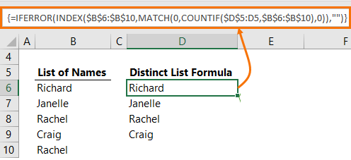
Here is the formula so you can copy it to your own workbook:
=IFERROR(INDEX($B$6:$B$10,MATCH(0,COUNTIF($D$5:D5,$B$6:$B$10),0)),"")
Notes:
- The formula must start at least one row below row 1
- The source data cannot contain any empty cells.
- The range in COUNTIF starts 1 row above the cell containing the formula. i.e. in this case D5 - if your formula starts in a different row then you need to adjust this reference accordingly.
- This is an array formula, so it must be entered with CTRL+SHIFT+ENTER. That’s how the curly braces are inserted that you can see in the formula bar.
- Copy the formula down.
What’s that? You want a sorted list. Ok, you can use this formula:
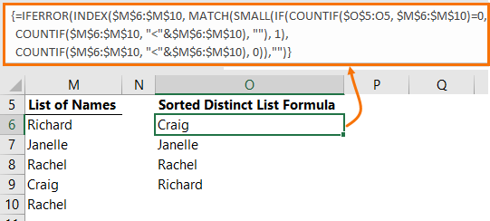
Here is the formula so you can copy it to your own workbook:
=IFERROR(INDEX($M$6:$M$10, MATCH(SMALL(IF(COUNTIF($O$5:O5, $M$6:$M$10)=0, COUNTIF($M$6:$M$10, "<"&$M$6:$M$10), ""), 1), COUNTIF($M$6:$M$10, "<"&$M$6:$M$10), 0)),"")
Notes:
- The formula must start at least one row below row 1
- The source data cannot contain any empty cells.
- The range in the first COUNTIF starts 1 row above the cell containing the formula. i.e. in this case D5 - if your formula starts in a different row then you need to adjust this reference accordingly.
- This is an array formula so it must be entered with CTRL+SHIFT+ENTER
- Copy the formula down.
Now normally I’d translate those formulas into English, but I’m not going to waste your time or mine because I don't recommend this approach. There are less complicated and more robust ways to extract a list of unique values, namely Power Query or PivotTables, that I cover below.
Pros: Automatically updates when new data is added to the range….assuming the range being referenced in the formula is an Excel Table or dynamic named range so that it too expands to include the new data. The example above doesn’t reference dynamically expanding ranges.
Cons: These are complex formulas that are easily broken if an unsuspecting user edits the cell and doesn’t enter it with CTRL+SHIFT+ENTER. Array formulas can slow workbooks down, especially if the range being referenced is large, or there are lots of these formulas.
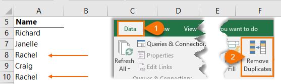
Remove Duplicate Values
A quick and easy way to get a list of unique values is to take a copy of the column of data for which you want to get the list, then Data tab > Remove Duplicates
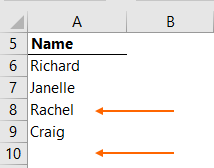
And I’m left with a list of unique values:
Pros: Quick and easy to use.
Cons: If your data gets updated then you need to copy the source column and run the Remove Duplicates process again.
Extract Unique Values with Advanced Filter
Advanced Filter can extract a list of unique items from a column or columns. First select the data, then Data tab > Advanced:
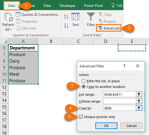
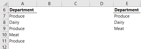
In the Advanced filter dialog box (image above) choose to copy the list to another location (4 & 5), and check the box for ‘Unique records only’. And voila, we now have two lists, the original, and the list of unique values in column E:
Pros: Easy to use.
Cons: No link is maintained between the original data and the filtered data. If the original data gets updated then the Advanced Filter must be run again.
Extract a Unique List with PivotTables
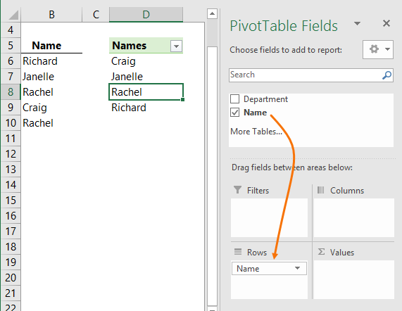
A PivotTable is an excellent way to quickly extract a list of unique items which can then be used to feed Data Validation lists etc.
Simply place the column you want the list for into the Rows area:
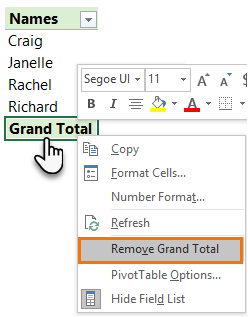
Tip: Right-click the Grand Total cell > Remove Grand Total:
Pros: Quick and easy to do. It automatically sorts the list in alphabetical order and it retains a connection to the source data so it’s easy to refresh/update. Unlike formulas, PivotTables are not easily broken.
Cons: Requires clicking on the Refresh button to update the PivotTable, or you can write some VBA code to automatically refresh it.
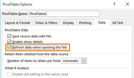
Tip: Set the PivotTable Options to refresh upon opening of the file:
Tip: Use a dynamic named range to reference the list in the PivotTable and use it in other formulas, or data validation lists.
Power Query Extract Unique Values from Column
Power Query (available in Excel 2010 onwards), has a Remove Duplicates tool, which essentially leaves you with a list of unique values.
Format your data in an Excel Table then load the data into Power Query:
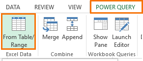
Excel 2010 & 2013: Power Query tab > From Table:
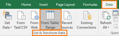
Excel 2016: Data tab > Get & Transform group: From Table:
This will load a copy of the data into Power Query and launch the Power Query Editor window.
In the Power Query Editor simply select the column you want it to extract a unique list from > right-click > Remove Other Columns (assuming there is more than one column in your table).
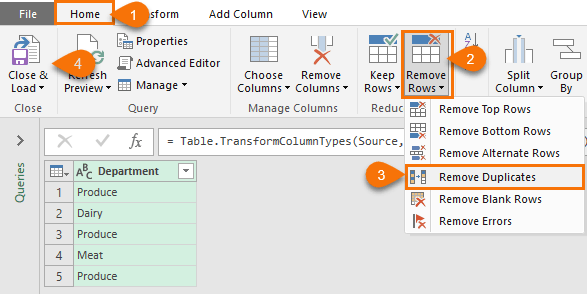
Then Home tab (1) > Remove Rows (2) > Remove Duplicates (3):
Tip: before closing and loading, click the filter button for the column and sort the data.
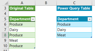
Click Close & Load (4) > to Table. Now you have two tables; your original table and your Power Query table containing the unique list:
Pros: The great thing about using Power Query is if your source data gets updated you can Refresh the query and it will remove duplicates again. No need to open the query editor. The original data remains intact.
Tip: You can link a Data Validation list to a Power Query table and it will automatically pick up new data. No need to create a dynamic named range like you have to with PivotTables.
Cons: Requires a few more steps than the PivotTables. Power Query is not available in Excel 2007.
Highlight Unique Values with Conditional Formatting
You don’t always want to extract a list of unique values, sometimes you might just want to highlight them. Conditional Formatting can quickly highlight duplicates in a column. Simply select the column of cells containing the suspected duplicates > Home tab > Conditional Formatting > Highlight Cells Rules > Duplicate Values:
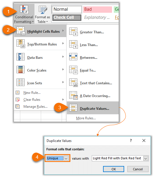
Tip: You can change the format by clicking the drop down for ‘Values with’ (see image above).
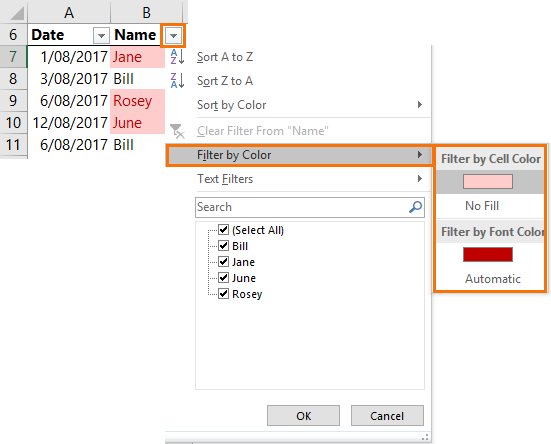
Once the formatting is applied you can use filters (Data tab > Filters), based on the cell fill color or font color to display or hide the duplicate values:
Pros: Great for visually highlighting unique values in a column. You can use filters to hide or focus on unique values or duplicate values.
Cons: Duplicates do not get highlighted at all, so you can’t use the formatting to display a unique or distinct list. This technique doesn’t highlight the row and only identifies unique values in a single column.
Highlight Unique Rows with a Conditional Formatting Formula
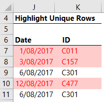
Let’s say you want to highlight rows that contain unique values across a row. For example, rows 7, 8 and 10 have the unique Dates and ID’s:
For this we need to apply the conditional formatting using a formula:
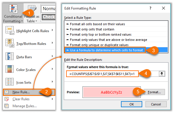
Click here for an in depth understanding of how to write formulas for conditional formatting.
Pros: highlights the whole row and takes into consideration more than one column. Filters can be used to hide the duplicates, or the unique values from view.
Cons: The formula can be difficult to remember. Duplicates do not get highlighted at all, so you can’t use the formatting to display a unique or distinct list.
So, there you have 6 ways to identify or extract a list of unique values. Depending on my needs I like to use Power Query or PivotTables to extract a distinct list, or Conditional Formatting to visually indicate unique records.
Dynamic Arrays - Office 365 [UPDATE]
If you have Office 365 then you can use the new simplified dynamic array UNIQUE function, and if you want to sort the unique list, you can use the SORT Function.
Related Lessons
Tutorials:
- Conditional Formatting
- Conditional Formatting with Formulas
- Advanced Filters
- Advanced Filter Unique Records
- Excel Tables
- PivotTables
Courses:

I have a column with 30k rows of IDs with a total of 45 unique IDs. I would like to add this formula so everytime I copy and past data on the IDs column, the formula will show me just the unique IDs on a separate column.
IDs Data is in B5:B30005 (B5 is the header)
In D6 I m inputting the following formula:
=IFERROR(INDEX($B$6:$B$30005,MATCH(0,COUNTIF($D$5:D5,$B$6:$B$30005),0)),””)
And it is not working as it should
Hi Dave,
Are you entering the formula with CTRL+SHIFT+ENTER as opposed to just ENTER?
Mynda
what if you want to filter by the largest to greatest instead of a~z
Hi,
I guess you mean sorting rather than filtering? And I’m not sure what you mean by ‘largest to greatest’? Isn’t that the same thing? You haven’t given any context, so I’m going to assume you have Dynamic Arrays and you are sorting numbers in A1:A10.
Sort in ascending order
=SORT(A1:A10)
Sort in descending order
=SORT(A1:A10,,-1)
Regards
Phil
{=IFERROR(INDEX(SORT, MATCH(LARGE(IF(COUNTIF($B$20:B20, SORT)=0, COUNTIF(_2019, “<"&_2019), ""), 1), COUNTIF(_2019, "<"&_2019), 0)),"")}
I wrote this formula but it seems to not go thru the whole list of names… I have close to 600 customer but it only sorts to lik 90 and the rest just list of a single customer name… I don't really know what the formula is doing but… i feel like i missing something in the formula…
Hi,
Please start a topic on our forum and attach your workbook. It’s too easy to make mistakes if we have to recreate the data you are working with.
Regards
Phil
how do i do that?
PLS also note that the data I’m working with is very huge
From the menu at the top of the site. Forum -> Register as Forum Member.
Then read the Forum Rules and Guides to see how to post a question and attach files.
Regards
Phil
=IFERROR(INDEX($B$6:$B$10,MATCH(0,COUNTIF($D$5:D5,$B$6:$B$10),0)),””) works but one needs to figure out how many distinct values are going to exist in order to copy and paste the formula that many times. Hence, if there are 10 distinct values then one copies and paste the formula 9 times. Is there a way for one does not need to know how many distinct values are going to exist?
Hi Cal,
The formula already has error handling, so you can simply drag it down further than you need, allowing for growth in the list.
Mynda
Hi I have an sheet with three column First Colum having some drug names, second having manufactured date, third having expiry date. I want to get list of drug names which are manufactured and not expired on the date entered a cell of another sheet.Or Simply want to filture out few list of items on some conditions on another cell
Hi Jaigopal,
This can be done quite easily with Advanced Filter or adding a helper column and using the filter drop downs on a Table. If you post your question and sample Excel file on our forum we can give you a specific answer with an example.
Mynda
In my experience, the simplest formula would be a vlookup with fixed starting point and moving end. If this returns an error, then the value is unique. So this must be used in conjunction with If(iserror(),TRUE,FALSE) so as to capture a TRUE and FALSE value. FALSE =””.
Hi Rolan,
I’m not seeing how that would work. But now that we have Dynamic Arrays the simplest formula uses the UNIQUE function e.g. =UNIQUE(range)
Mynda
Hello Mynda,
My non-array formula for the sorted distinct list starting in Cell N6, copied down to Cell N10, is this:
=IFERROR(LOOKUP(2,1/(COUNTIF(M$6:M$10,”>=”&M$6:M$10)=MAX(INDEX(
COUNTIF(M$6:M$10,”>=”&M$6:M$10)*(COUNTIF(N$5:N5,M$6:M$10)=0),0))),
M$6:M$10),””)
Thanks for sharing, Robert!
Regarding: =IFERROR(INDEX($B$6:$B$10,MATCH(0,COUNTIF($D$5:D5,$B$6:$B$10),0)),””)
How can I extend this to cover two columns of source data?
Hi Mark,
instead of returning a null string at the iferror argument, use the same formula with the second column:
=IFERROR(IFERROR(INDEX($B$6:$B$10, MATCH(0,COUNTIF($D$5:D5,$B$6:$B$10),0)), INDEX($C$6:$C$10, MATCH(0,COUNTIF($D$5:D5,$B$6:$B$10),0))),””)
ok it works. Turns out your “” from the reply were causing the issue. Any idea how to remove/ignore empty cells?
See:
https://www.myonlinetraininghub.com/excel-remove-blank-cells-from-a-range
https://www.myonlinetraininghub.com/excel-ignore-blanks-in-data-validation-list
They should be what you need.
Regards,
Catalin
previous one worked fine. no two last questions –
1. how to ignore empty cells
2. how to ignore specific value (text) of the cell?
1 and 2 are separate functions
Hi Mark,
in case you missed it, I already sent a link to an article describing how to ignore empty/blanks.
I suggest using power query solution to solve all the problems, including removing duplicates, sorting the final list, ignoring specific values, complex formulas may be difficult to maintain.
Very useful tools and formulas…
Thanks 🙂
Thanks, Irfan!
Is there any way to modify the formula in “Excel Formula to Extract a List of Unique Values from a Column” to work with empty cells? In other words I would like a sorted unique list of only non-blank cells.
Hi PB,
No need to change this formula, try this article about removing blanks from a range, it will not remove duplicates.
Wow!! This was amazing!!! I immediately had to share these functions with my coworkers! Thank you Mynda!!
Thanks Samuel, glad it was useful for you.
5. Then highlight the range you’re looking to fill and Fill, Down. (Highlighting the range and F2, CNTL+SHIFT+Enter doesn’t work)
Hi Keith,
Where do I mention step 5?
Mynda
How would you combine this with criteria from a validation list? Ex: Store A in validation list uses formula to extract a list of unique values from a column (sales reps)?
Hi John,
In the downloadable file, there are examples for 6 ways to extract unique values. At least one of them will take additional criteria, Power Query can take any number of criteria you want, but depends on your specific needs.
If you can’t make any example work, please upload a sample file on our forum to see your structure. (create a new topic)
Catalin
Thank you very much Mynda for sharing these valuable insights! I can’t wait to receive your fantastic tips every week.
I would like to ask you how the COUNTIF function works in the formula.
Hi Juan,
The COUNTIF function is counting the number of times a name in the range of cells above the current cell (in column D) is found in the ‘List of Names’ in column B. The MATCH function is looking for names that aren’t already in the distinct list, hence it’s looking for a zero count. When COUNTIF doesn’t find the name it returns zero, which is a ‘MATCH’. The position of that match is given to INDEX so it knows which name to return next. However, if the COUNTIF finds a name in column D that is in the list of names in column B it will return 1, and so it will be ignored.
Mynda
Thank you very much Mynda for the reply, now the formula is beginning to make sense for me. It’s very creative to combine these functions to create a formula that allows to achieve this result, great!
I have another question about the second formula: what’s the meaning of this formula combined with SMALL function: COUNTIF($M$6:$M$10, “<"&$M$6:$M$10)?
Hi Juan,
The COUNTIF tells SMALL which is the next name to return. It’s what enables the names to be sorted. If you use the Evaluate Formula tool on the Formula bar you can see how it evaluates. That should help you understand how it’s working.
Mynda
Thank you Mynda. I tried to evaluate the formula COUNTIF($M$6:$M$10, “<"&$M$6:$M$10) and the result is {4;1;2;0;2}. I do not understand well what it means. The fourth name of the result is Craig and it's sorted in the first place in the new list, I suppose that's the meaning of the first "4". But the "1" number does not reflect the position of the next name of the range M6:M10 in the new list.
I am amazed how you achieved to create such a complex formula! That requires a lot of critical thinking 😮
Hi Juan,
You can’t just look at the COUNTIF part of the formula in isolation, you have to read the whole formula to make sense of how it works. Here is the formula in cell O6:
It says index the range M6:M10, match the smallest value that hasn’t already been returned and return it, but if there’s an error, return blank. The first COUNTIF checks if a name has already been returned, if it has been returned i.e. it’s already in the list in column O, then “” is input into the array returned by COUNTIF so that this name can be skipped.
The second and third COUNTIF formulas return the order of the names. {4;1;2;0;2} with 4 being the last name to return (i.e. Richard), and zero being the first name (i.e. Craig). SMALL looks for the smallest name still present in the array. If the name has already been listed then it will have “” in it’s position so small will pick up the next name.
Looking at cell O6 it evaluates like so:
=IFERROR(INDEX($M$6:$M$10, MATCH(SMALL({4;1;2;0;2}, 1),{4;1;2;0;2}, 0)),"")=IFERROR(INDEX($M$6:$M$10, MATCH(0,{4;1;2;0;2}, 0)),"")Whereas looking at cell O7 it evaluates like so (notice the 0 for Craig in the first array is now “” because it was found in the first COUNTIF):
=IFERROR(INDEX($M$6:$M$10, MATCH(SMALL({4;1;2;"";2}, 1), {4;1;2;0;2}, 0)),"")=IFERROR(INDEX($M$6:$M$10, MATCH(1, {4;1;2;0;2}, 0)),"")The complexity of this type of formula is exactly why I don’t recommend you use it. There are simpler ways to achieve the same results, so why go down a path that’s unnecessarily complex.
Mynda
Thank you very much Mynda for the explanation. It is still very difficult to understand how it works.
It would be interesting to develop a course on how to order the ideas to create such nest formulas, strategies to use to combine multiple functions