Excel Advanced Filters

To be honest I don’t use Advanced Filters much. I tend to use the regular AutoFilter, or if I need more I’ll use the Custom AutoFilter. Not because they’re necessarily better, it’s probably more out of habit than anything else.   But Advanced Filters have a couple of advantages over regular filters:  

1. The filter criteria is contained on your worksheet so you can easily see what filters are applied. Whereas with AutoFilter you have to click on the down arrow to see what filters have been applied.
2. Advanced Filters allow you to extract your filtered data to another place in your worksheet/workbook or extract a unique list of records.

Their downside is it’s not as obvious that your data is filtered since they don’t display drop-down lists for the column headers like regular filters.

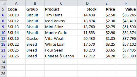
Take this list below that has an Advanced Filter applied as an example. The only tell-tale sign that some of the data is hidden are the blue row numbers.

How to use Advanced Filters

Make Space for Your Criteria

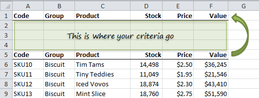
First of all you need to house your criteria (the rules for your filter) somewhere on your worksheet. I like to put it above my data for two reasons:

1. It’s in a nice obvious place which will hopefully remind me or other users that a filter is applied (in case those blinding blue row numbers don’t catch my eye!).
2. Your criteria must have a header row just as your table of data has and they must be exactly the same (except it’s not case sensitive), so I find it easy just to copy and paste the column headers from my data table for my Criteria range. Note: you don’t have to represent every column in your Criteria, but since I only have a few columns it’s just as easy to copy them all at this stage.

So go ahead and insert a few rows above your data and copy and paste your column headers like this:

Enter Your Criteria

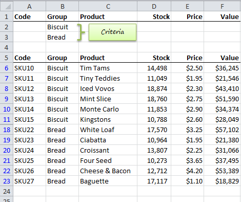
Let’s start with any easy one and filter any records that have the text Biscuit OR Bread in the Group column. We do this by listing each of our criterion in separate cells under the corresponding heading in our Criteria range:

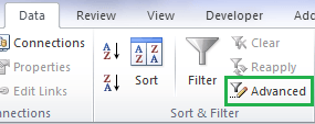
Now to apply the Advanced Filter place your cursor anywhere in your data table (this helps Excel detect your ‘List range’) > click on the Advanced Filter icon on the Data tab of the ribbon.

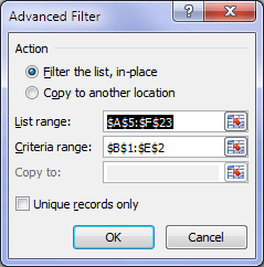
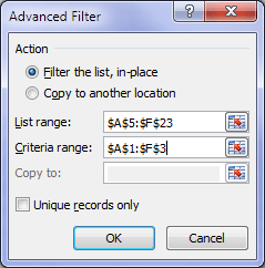
This will open the Advanced Filter dialog box:

Make sure your 'List range' and 'Criteria range' are correct and click OK.

Tips:

1. If you want to extract a list and copy it to another place in the existing worksheet simply select the ‘Copy to another location’ button and tell Excel where you want to ‘Copy to’. Note: if you want to copy it to a different worksheet follow these instructions.
2. Make sure you don’t select any blank rows in your criteria range otherwise your filter won’t work.
3. The first time you apply an advanced filter Excel creates a named range for your criteria called…wait for it….’Criteria’. The only problem with it is that it doesn’t grow/contract as you add or remove criteria. However, you can edit it in the name manager and make it a dynamic named range.

Advanced Criteria

Moving on…. the example above looks at how entering two or more criteria for one column is the same as the OR logic you might already be familiar with.  i.e. Group = Biscuits OR Group = Bread.

Let’s look at some other scenarios.

AND Logic

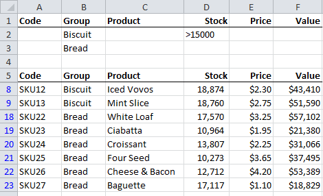
The criteria in the image below reads:

Filter data where Group = Biscuit AND Stock > 15000 OR Group = Bread.

Criteria entered on the same row is treated as AND, whereas criteria entered in the same column is treated as OR.

OR Criteria for Multiple Columns

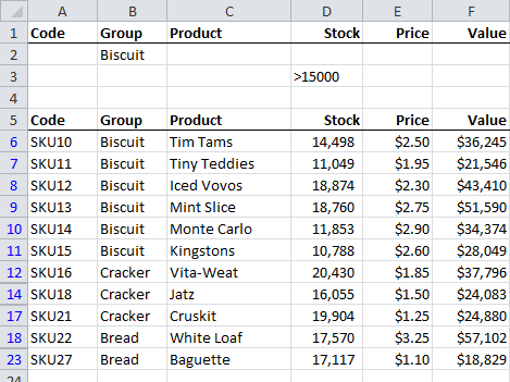
The criteria in the image below reads:

Filter data where Group = Biscuit OR Stock >15000

We can see that the data is displaying all of the Biscuit data as well as Cracker and Bread records where their Stock is >15000.

Greater Than AND Less Than

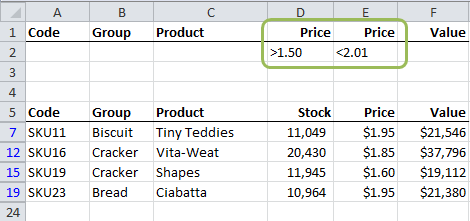
The criteria in the image below reads:

Filter the data where the Price is greater than $1.50 AND less than $2.01.

Note how I have two ‘Price’ columns in my Criteria.

Using Wildcards in your Criteria

You can get creative with your criteria and employ wildcards to allow broader searches or be more specific.

Using Formulas in your Criteria

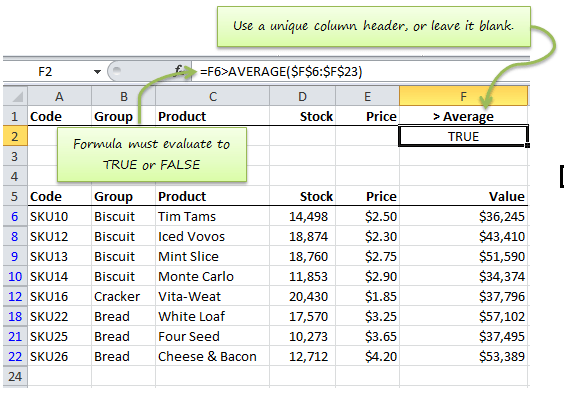
Let’s say we want to filter all Values that are greater than the average Value.

The reference to F6 in the formula =F6>AVERAGE($F$6:$F$23) is simply the first row of the data range I want to base my filter on.

Case Sensitive Filters

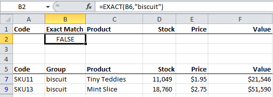
Case sensitive filters are just another type of Formula Criteria that evaluates to TRUE or FALSE. To perform a case sensitive filter you use the EXACT function like this:

Notes:

1. The criteria label in this example is ‘Exact Match’, not ‘Group’ like you might expect. You could leave the criteria label blank or give it a different name, but it can’t be Group or any other column label from your data table.
2. As with the formula criteria, the reference to B6 in this formula =EXACT(B6,"biscuit") is also the first row of the data range I want to base my filter on.

Filtering Specific Text

In all of the examples above (except Case Sensitive filters), I have entered the Group criteria by typing the name in the cell like so; 'Biscuit', 'Bread' etc.

But if you have several groups that all contain the word  ‘biscuit’ in their name e.g. Biscuit, Biscuit Savoury and Biscuit Sweet , then Excel will display all 3 since they all start with the word ‘biscuit’.

However, if you want to filter the records for an exact match you can use the EXACT function as I did above or you can enter your criterion like this:

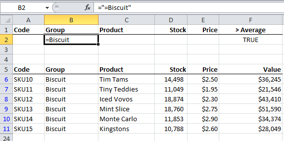
="=biscuit"

See how in the cell B2 Excel only displays the portion of the text in the double quotes but in the formula bar you can see I have entered ="=biscuit":

What Do You Think?

If you liked this please share it with your friends on Facebook, Twitter, LinkedIn or +1 on Google using the buttons below, or leave me a comment and tell me what you use Advanced Filters for.