The Excel SORT function sorts the contents of a column, columns (range) or array in ascending or descending order. The syntax is:
=SORT(array, [sort_index], [sort_order], [by_col])
array is the range or array containing the values you want sorted.
sort_index is optional and indicates the row or column to sort by. When omitted it will default to sort by the first row or column in the array.
sort_order is optional. It’s a number; 1 for ascending and -1 for descending. If omitted, it will sort in ascending order.
by_col is an optional logical value (TRUE/FALSE) indicating the desired sort direction; FALSE to sort by row (default), TRUE to sort by column. Most of the time you’ll want to sort by row.
Note: The SORT function is part of the new Excel Dynamic Arrays family and at the time of writing, Dynamic Arrays are only available in Office 365 and are currently in beta on the Insiders channel. Excel 2019 will not have the Dynamic Array functions.
Excel SORT Function Examples
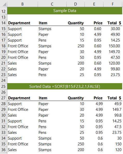
Let’s say we want to sort the table in cells B15:F23 based on the Item column (C). We can use the SORT function like so:

The formula, =SORT(B15:F23, 2, 1, FALSE) translates in English to:
Sort the data in cells B15:F23, based on the second column, in ascending order, sorted by row.
Sort a Distinct List
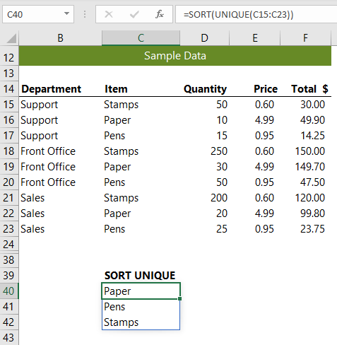
I expect one of the most common uses for SORT will be to sort a UNIQUE List. In the example below, I’ve used the UNIQUE function to extract a list from the Items in column (C), and then wrapped it in the SORT function:

Notice I’ve omitted the optional sort_index, sort_order and by_col arguments as the default is to return a list sorted based on the first column in ascending order by row.
Data Validation using Sorted Unique List
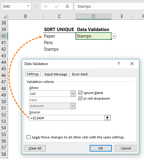
We can easily use the sorted unique list in a data validation list by using the spilled range operator, #, like so:

By using the spilled range operator the data validation list will automatically adjust the results to match the spilled range as it grows or contracts.
Sort Multiple Columns
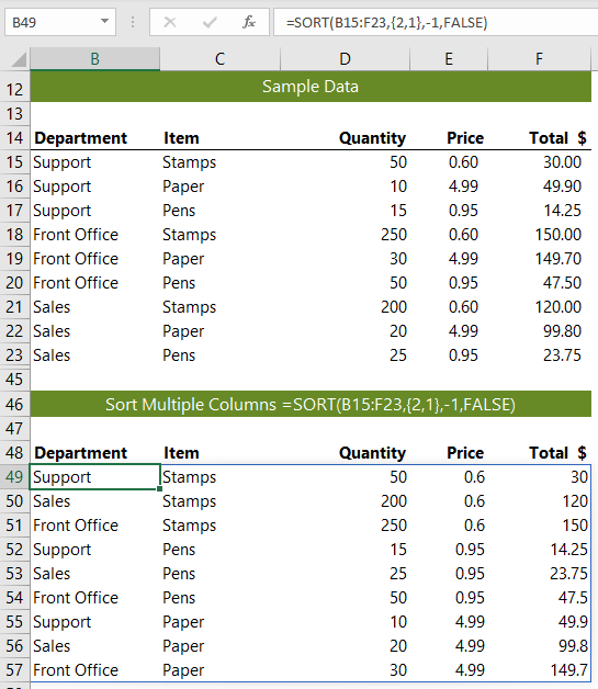
Let’s say you want to sort by Items and then by Department in descending order. You can pass an array of sort_index arguments by surrounding them in curly braces and then separating them with a comma, as shown below:

Tip: If you want to sort one column in ascending order and another in descending order you can pass an array of sort_order arguments like this:
=SORT(B15:F23,{2,1}, {1,-1}, FALSE)
Thanks to Bill Jelen, aka MrExcel for sharing that last example.
Download the Workbook
Enter your email address below to download the sample workbook.
Related Tutorials
| Excel FILTER Function | Filter cells based on criteria. |
| Excel RANDARRAY Function | Returns an array of random numbers between 0 and 1. |
| Excel SEQUENCE Function | Returns list of sequential numbers that increment as specified. |
| Excel SORTBY Function | Sort cells or arrays based on criteria. |
| Excel UNIQUE Function | Extract a unique or distinct list from a range or array. |