Excel FILTER Function

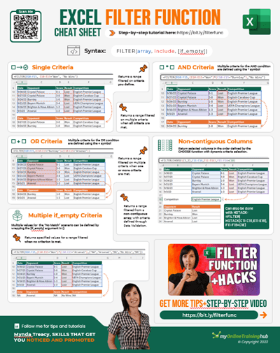
The Excel FILTER function returns a range filtered on criteria you define. It can also handle multiple AND/OR criteria.

FILTER Function Syntax

=FILTER(array, include, [if_empty])

array is the range or array containing the values you want filtered.

include is the logical test that returns a Boolean array (TRUE/FALSE)  the same height or width as the array.

if_empty is an optional value to return if the included array are empty i.e. if the filter results in no records.

Note: The FILTER function is part of the new Excel Dynamic Arrays family. At the time of writing, Dynamic Arrays are only available in Microsoft 365. Excel 2019 will not have the Dynamic Array functions.

Watch the Video

Download the Workbook

Excel FILTER Function Examples

Let’s say we want to filter the table in cells B14:F22 for the Sales Department and if there are no matching records return the text ‘No Records’. You can see the results of the FILTER function has ‘spilled’ creating a new table in cells B27:F29 below:

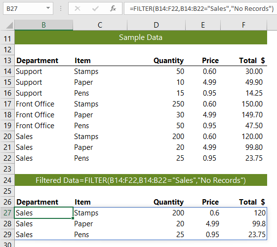
The formula; =FILTER(B14:F22,B14:B22="Sales","No Records") reads in English:

Filter the cells B14:F22, where the values in cells B14:B22 contain "Sales", if no matches are found then return the text “No Records.

Excel FILTER Functions using AND Criteria

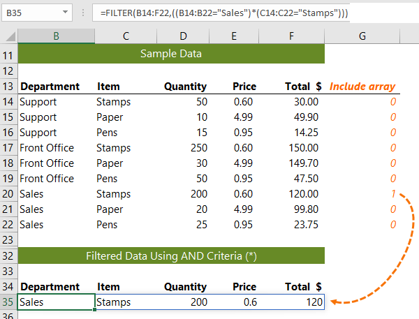
We can add multiple criteria to the include argument by surrounding them in parentheses and using the multiplication operator as shown below:

The formula in B35; =FILTER(B14:F22,((B14:B22="Sales")*(C14:C22="Stamps"))) evaluates like so:

=FILTER(B14:F22,
  (
  {FALSE;FALSE;FALSE;FALSE;FALSE;FALSE;TRUE;TRUE;TRUE} *
  {TRUE;FALSE;FALSE;TRUE;FALSE;FALSE;TRUE;FALSE;FALSE}
  )
)

Two sets of TRUE and FALSE Boolean values are multiplied, which converts them to their numeric equivalents of 1 and 0, resulting in the final include argument array:

=FILTER(B14:F22,({0;0;0;0;0;0;1;0;0}))

Only one record matches both criteria, and this is returned by the FILTER function:

Tip: You can add more AND criteria to the ‘include’ argument by following the same pattern of surrounding the criteria in parentheses and multiplying it by the existing criteria.

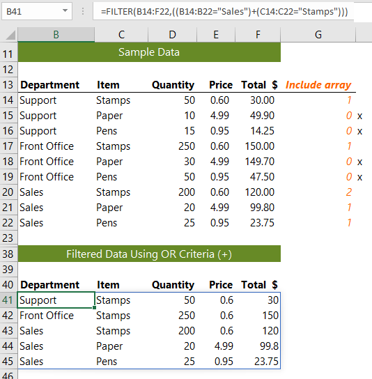
Excel FILTER Functions using OR Criteria

Similarly, we can filter using OR criteria by using the + operator as shown below:

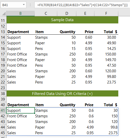
The formula in B41; =FILTER(B14:F22,((B14:B22="Sales")+(C14:C22="Stamps"))) evaluates like so:

=FILTER(B14:F22,
  (
  {FALSE;FALSE;FALSE;FALSE;FALSE;FALSE;TRUE;TRUE;TRUE} +
  {TRUE;FALSE;FALSE;TRUE;FALSE;FALSE;TRUE;FALSE;FALSE}
  )
)

The two sets of TRUE and FALSE Boolean values are added together, which converts them to their numeric equivalents of 1 and 0, resulting in the final include argument array:

=FILTER(B14:F22,( {1;0;0;1;0;0;2;1;1}))

The rows with a zero are excluded from the Filter:

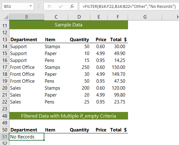
FILTER Function with Multiple If_Empty Criteria

The standard way to use the if_empty argument is to return a single value, like in the example below which returns the text ‘No Records’:

However, you can return a different result for each column by adding them with a comma separator and surrounding them in curly braces, as shown below:

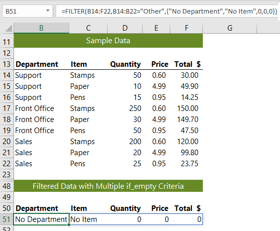
Thanks to Bill Jelen, aka MrExcel for that last tip.

FILTER and Rearrange Non-contiguous Columns

We can use the CHOOSE function to specify the columns we want to filter and rearrange their order:

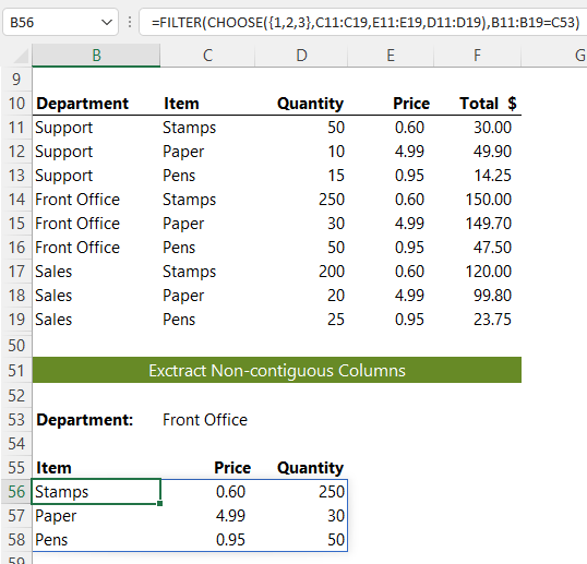
We can also link the criteria to a data validation list (see cell C53) making it dynamically update

Related Excel Functions

Excel RANDARRAY Function	Returns an array of random numbers between 0 and 1.
Excel SEQUENCE Function	Returns list of sequential numbers that increment as specified.
Excel SORT Function	Sort cells or arrays in ascending or descending order.
Excel SORTBY Function	Sort cells or arrays based on criteria.
Excel UNIQUE Function	Extract a unique or distinct list from a range or array.