Excel AGGREGATE Function

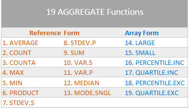
The AGGREGATE Function is the Swiss Army Knife of functions; it’s so versatile it can replace these 19 Excel functions in one fell swoop:

But that’s not reason enough to use it, the function-killer reason to use AGGREGATE over any of the 19 standard functions it can replace is because it is far more powerful.

Download the Excel File

Excel Aggregate Function Video

Excel AGGREGATE Function Options

You see, the second argument of the AGGREGATE function is ‘Options’, which enables you to tell it how to handle hidden rows, error values, and nested SUBTOTAL and AGGREGATE functions by specifying an option number from the list below:

AGGREGATE can handle Arrays

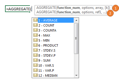
AGGREGATE has two forms, Array ¹ and Reference². You’ll notice when you type in the function that you have a choice (kind of):

The ‘form’ is dictated by the function_num you choose. Functions 1 to 13 are Reference form and 14 to 19 are array form.

AGGREGATE in Reference Form

Let’s look at how it compares to the SUM function, which means we’ll use the Reference form, as SUM is function_num 9.

The syntax:

=AGGREGATE(function_num, options, ref1, …)

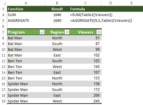
My data is in an Excel Table called ‘Table1’, so I’m using the table Structured References in my formula. e.g. Table1[Viewers] refers to cells C8:C19.

I’ve used Option number 5, which ignores hidden rows (which really means rows hidden by a filter as rows hidden manually are ALWAYS ignored). And you can see in the image below that when there are no rows hidden both formulas return the same result (cells B4 and B5):

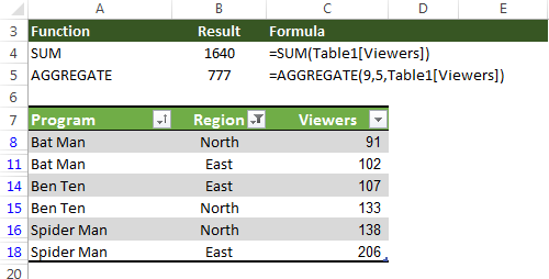
However when I hide some rows, by filtering out the South and West regions, my AGGREGATE formula returns a result that ignores the hidden rows, whereas SUM still includes the hidden rows:

AGGREGATE in Array Form

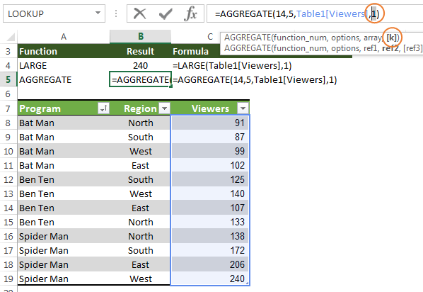
Similarly we can find the largest value in the Viewers column with function_num 14 for LARGE.

This means we’re using AGGREGATE in array form. And notice we also have an extra argument to specify ‘k’, with 1 returning the largest, 2 returning the second largest and so on:

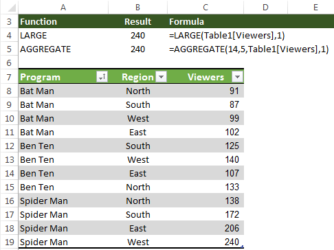
With no rows hidden LARGE and AGGREGATE return the same result (see below):

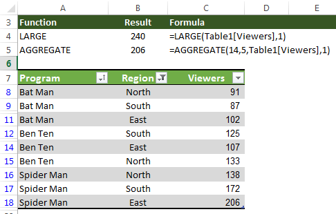
But with rows for West hidden we get different results with AGGREGATE, as you can see below (note; I've used option number 5 - ignore hidden rows in AGGREGATE):

Tip: with dynamic arrays we can also use AGGREGATE to spill results. For example, let's say we want to return the top 2 results. We can use this formula:

=AGGREGATE(14,5,Table1[Viewers],{1;2})

Exploiting Option 6 – Ignore Hidden Rows and Error Values

So far, we’ve only looked at Option number 5, which ignores hidden rows. Option number 6 allows us to ignore error values, and we can use this to our advantage to only aggregate values that meet a certain condition, or criteria.

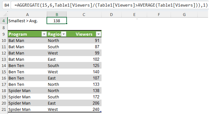
For example, let’s say we want to identify the smallest value that's greater than the average of the entire list. With AGGREGATE we can use the SMALL function_num 15, like so:

Let’s take a closer look at this formula above and how it evaluates:

=AGGREGATE(15,6,Table1[Viewers]/(Table1[Viewers]>AVERAGE(Table1[Viewers])),1)

The array argument takes the values in the Viewers column and then uses Boolean logic Table1[Viewers]>AVERAGE(Table1[Viewers]) to test if the values are above average.

When Table1[Viewers]>AVERAGE(Table1[Viewers]) is evaluated it returns a series of TRUE and FALSE values like this:

=AGGREGATE(15,6,Table1[Viewers]/{FALSE;FALSE;FALSE;FALSE;FALSE;TRUE;FALSE;FALSE;TRUE;TRUE;TRUE;TRUE},1)

In Excel when a math operation is performed on a logical value (TRUE or FALSE), they are converted to their numeric equivalent of 1 and 0.

So when the Table1[Viewers] array is expanded Excel divides them by the values in the logical test array which converts them to 1 and 0:

=AGGREGATE(15,6, {91;87;99;102;125;140;107;133;138;172;206;240}/ {0;0;0;0;0;1;0;0;1;1;1;1},1)

And when we divide anything by zero we get an error, so our formula is littered with #DIV errors for values in the Viewers column where the values is below average, like this:

=AGGREGATE(15,6,{#DIV/0!;#DIV/0!;#DIV/0!;#DIV/0!;#DIV/0!;140;#DIV/0!;#DIV/0!;138;172;206;240},1)

Have you worked out where I’m going with this? Remember the Option number argument of 6 ignores errors, so AGGREGATE now looks like this with all the #DIV errors gone:

=AGGREGATE(14,6,{140;138;172;206;240},1)

And the smallest value is:

=138

If the concept of arrays is hurting your head and you want to learn more about array formulas (I don’t know, you might be a glutton for punishment ;-)), then check my Advanced Excel Formulas Course.

AGGREGATE Notes:

1. As with many Excel functions, AGGREGATE is designed to work with data in columns, so when you reference a horizontal range, AGGREGATE will not ignore values in hidden columns. It only ignores hidden rows in a vertical range.
2. You might have noticed AGGREGATE is similar to the SUBTOTAL function in that it can perform a range of different calculations, and you’d be right, but I’m sure you’ll agree that AGGREGATE is much more powerful.
3. AGGREGATE will not ignore filtered rows, nested subtotals or nested aggregates if the array argument includes a calculation, as it does in the last example (=AGGREGATE(15,6,Table1[Viewers]/(Table1[Viewers]>AVERAGE(Table1[Viewers])),2). i.e. option numbers 0 through 5 and 7 will not ignore filtered rows.
4. AGGREGATE will always ignore rows hidden manually i.e. using right-click > hide when using any of the option numbers that ignore hidden rows. If you don't want to ignore rows hidden manually, use the SUBTOTAL function.