Excel Filters are right at home with large tables of data.
You can use them to limit the data displayed in your table to only that which meets one or more criteria you specify.
When your data is filtered Excel hides the rows that do not meet your criteria.
You can apply them to more than one column, with each additional filter being added to the current set to further reduce the data displayed.
For this tutorial I’ve borrowed some data from Phil (my husband).
You see Phil is a keen Eve fan. No, Eve is not another woman, although I do sometimes feel a bit widowed by Eve. Eve is an online sci-fi computer game where you fly fantasy space ships, in a fantasy galaxy, fighting fantasy battles to feed your obsession with geeky stuff.
I won’t bore you with anymore details on how the game works, other than to say there’s a lot of buying a selling of (fantasy) commodities and as a result the game generates large tables of data. Perfect for filters.
Inserting Excel Filters
1. First make sure your data is in a tabular format. That means there are column headings or labels, but no row labels, and preferably no blank columns within your table.
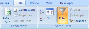
2. On the Data tab in the Ribbon go to the Sort & Filter section and click on the Filter button.
3. Down arrows will appear in each column heading like this:
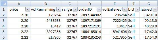
That’s it. You're ready to go!
How to Use Filters
You can create 3 types of filters:
1. by numeric values - available when the column contains numbers
2. by text that meets a certain criteria - available when the column contains text
3. by cells that meet a format style – available when the column has font or cell formats.
Clicking on any of the filter arrows opens a menu of tools where you can select from the different types relevant to the type of data in the column.
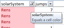
Note: The icon on the filter button changes when you have a filter in place.
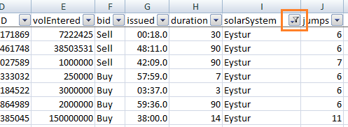
Tip: To see what filter is applied hover your mouse over the icon and a screen tip will appear.
Text Options
1. Sorting by A to Z and vice versa is as it suggests. Just be aware that once you select one of these sort options you cannot undo it.
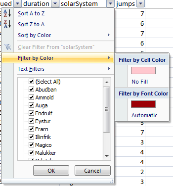
2. Sort by Colour is great if you’re using Conditional Formatting, or even if you just have different coloured text or cell fill.
3. By colour allows you to only display rows that meet the colour criteria you choose, whether it be the font colour or the cell colour.
4. Or simply tick or un-tick the items you want to filter from the list.
5. Text Filters (see menu below) allow you to specify criteria that matches a text value.
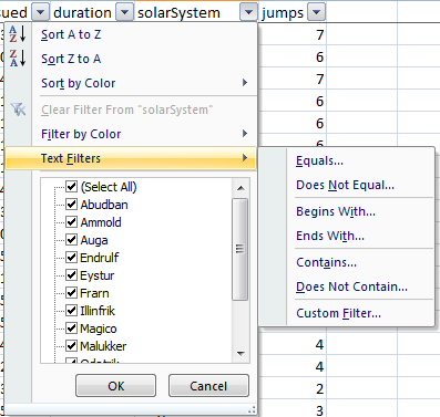
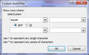
From the menu above I selected Text Filter > Equals and the window below opens to allow you to specify your criteria.
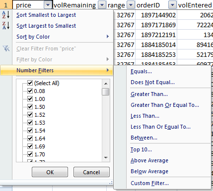
Number Options
If you select Filters on a number column (see image below) you get slightly different menu options, including Less Than, Greater Than, Top 10, and Averages to name a few.
Dates or Times
When you apply a filter on a column containing dates you are presented with different options in the menu (see image below)
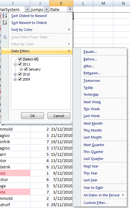
You will notice in the list that the dates are grouped by year, then month and so on.
You can either select specific dates from this list or you can select a time sensitive filter by clicking on Date Filters > and then selecting from the options available.
The time sensitive filters, like Today, Tomorrow, Next Month etc. are dynamic, meaning they will automatically update as time goes on. Each time you open the workbook Excel will reapply the filters based on the current date on your computer.
Tip: if you use a date filter it’s a good idea to format your dates. For example; if you’re filtering by month, format the date column as mmm-yy.
How to Apply a Quick Filter
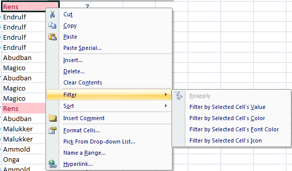
You can apply a quick filter based on the criteria that matches the active cell (see image below).
For example; my active cell below contains the text ‘Rens’ in a red font with pink fill. When I right click on the cell, and select Filter, Excel brings up a list of options based on the active cell.
How to Clear Filters
Simply click on the filter button and select ‘Clear Filter’.
Or to clear all click on the Data tab of the ribbon and select ‘Clear’ from the Sort & Filter group.
So, you can see from the options available in the windows above that there is a vast range of criteria you can specify. I recommend you have a play around with them. Since most of it is self explanatory I won’t bore you now.
Enter your email address below to download the sample workbook.
Warnings!
1. Summing filtered data with the SUM, COUNT, AVERAGE, MIN, and MAX formulas (and some others) results in Excel including both the hidden and visible cells in your formula. If you only want to sum the visible cells in a filtered set of data you need to use the SUBTOTAL Formula.
2. When you use the Find tool to search filtered data Excel will only search the data that is visible. To search all of your data you need to clear your filters.
3. Using the sort options in the filter is not reversible.
4. You cannot apply more than one filter to one column, they're mutually exclusive.
5. Make sure each column only contains one type of data. E.g. don’t have dates and text in the same column. The filter can only be applied to one type of data in each column.


hi, can we use “search” in the filter if we need to have more than one name for solar system appear. eg Filter solar system for Rens and Auga? Can we have more than 2 name using this function?
Thank you.
Estella
Hi Estella,
You can filter for up to 2 criteria if you use Filter > Text Filters and then specify OR in the dialog box. However, 2 is the maximum filter criteria using this method.
For more than 2 you need to use Advanced Filters.
Mynda
Your website has so many helpful tips, thank you!
I thought I was pretty confident with filters, but I’ve come across an issue with an inherited spreadsheet where the last row #1068 always appears, no matter which column I’m filtering on – in most cases it shouldn’t be showing. I’ve checked that there are no blank rows, no hidden rows, and the formatting of all rows is the same. I’ve removed the auto filter and put it back in different ways with no improvement. The data isn’t in an Excel Table.
Do you have any other ideas I can try please??
Thank you…
Hi Sarah,
Are you sure that the stubborn row is included in the filtered area? Try removing the filter, select the entire range and apply the filter.
Let us know if this was the case 🙂
Cheers,
Catalin
Now this is a spicy meatball!!! Never has drilling for the data to facilitate a quick report been easier! Not as fulfilling as a pivot table, but if you need data quick, this little trick can have a report on the bosses desk before his bellowing quits ringing….thanks for sharing and for making it so easy to understand. I have learned more from your site in the few months I’ve been here, than I have in…well, years! You are the best, and keep it coming!
Aw, thanks Tom. Glad you liked this ‘spicy’ tip 🙂
Mynda.
A filter can be applied on any column, but it is not easy to see which column has a filter applied. Can one cell be colour formatted if a filter is applied in that column, or can the drop down icon be colour formatted if that icon is being used?
Hi William,
You already have 3 visual indications that the Filter Mode is active: the drop down icon is different, the row numbers are blue, and you have filter results in Status Bar, like: “25 of 2300 records found”. The conditional formatting cannot be applied, and the column filter cannot be changed…
Catalin
superb
Thank you, Naresh 🙂
good please try again another one
Thanks, Naresh 🙂
AN TO QUOTE THE WORDS OF MY TEACHER THIS IS ONE REALLY HELPFUL SITE. 🙂
🙂 thank you, Boss.
Thank you for these pages, they are so helpful! I have some data that I would like to filter BY subtotals, is this possible?? Say I have several entries for each customer, and I want to ignore customers who have spent a total that is greater than a certain amount in future analyses…
Hi Dave,
If you use the Subtotals tool it automatically groups the data for you so that you can summarise the data by the subtotals etc. No need to use Filters too. See an example here:
https://www.myonlinetraininghub.com/how-to-insert-subtotals-in-excel
Kind regards,
Mynda.
If i have a data and if used filter maximum for find out raw by raw and i know , i required a macro for the particular data… will you pl help me out…. pl.. if you have any solution pl provide me…..
Hi Jltender Kumar,
Please send your file through HELP DESK.
I don’t see you will need a macro for this.
We have a built in function called
MAX.
for example, =MAX(A1:A45).
Cheers.
CarloE
the best lesson for excel filtering
Cheers, Aslam 🙂 Glad you liked it.
information was very useful. good
Cheers, Ravi 🙂
I find your tutorial extremely helpful. You wrote:
“First make sure your data is in a tabular format. That means there are column headings or labels, but no row labels, and preferably no blank columns within your table.”
I also immediately discovered that a blank row immediately below the filter row will cause problems.
Cheers, Kent. Thanks for pointing out another key rule for filters 🙂
great tips above
Thanks, Emmanuel 🙂
Thank you. It was so nice
Thanks
🙂 You’re welcome.
Thanks
You’re welcome 🙂
Excel Filter Warnings!
6. Reiterating what Mynda mentioned above regarding \no blank columns within your table\:
Filtering data with merged cells is not a good idea.
Helpful tips. Thanks.
Cheers, BC 🙂
thanks for the pdf.
You’re welcome 🙂
Thanks
Great
Thanks Tarun. I appreciate your feedback.