The MIN, MAX, SMALL and LARGE functions in Excel are fairly straight forward, but I’d like to show you a couple of tricks that won’t be obvious from reading the Excel help files.
First of all the syntax for MIN and MAX functions:
=MIN(number1, [number2],….)
=MAX(number1, [number2],….)
The ‘number’ can be keyed directly into the formula, or you can enter a cell range (e.g. B15:F15) or a range name.
Syntax for SMALL and LARGE functions:
=SMALL(array,k)
=LARGE(array,k)
Where the ‘array’ can be a cell range or a range name, and ‘k’ is the position in the array you want found.
Note the following formulas give the same result:
=LARGE(array,1) is the same as =MAX(number1,[number2]…) both return the biggest number.
=SMALL(array,1) is the same as =MIN(number1,[number2]…) both return the smallest number.
In these cases it is more efficient to use MAX or MIN as they require less computing by Excel.
Whilst this may not be an issue for small workbooks, if you work with large volumes of data, as is common when working with statistics, then you’ll want to preserve all your CPU for the more complex formulas.
MIN, MAX, SMALL, LARGE Examples
Let’s look at an example or each using the values below:

=MIN(B4:F4)
= 1
=MAX(B4:F4)
=7
=SMALL(B4:F4,2) i.e. the second smallest
= 2
=LARGE(B4:F4,2) i.e. the second largest
= 5
MIN and MAX Trick
What say we want to calculate when overtime occurs? We know that the normal hours per day are 7.5 and anything higher than that is deemed to be overtime.
We could set up a table like this:
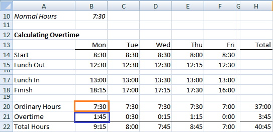
Where the formula in cell B20 for Ordinary Hours is:
=MIN($B$10,B22)
i.e. If B10 (normal hours) is smaller than B22 (total hours) then enter the value from B22 (total hours) in the cell, otherwise enter the value in B10 (normal hours).
And the formula in cell B21 for Overtime is:
=MAX(0,B22-$B$10)
i.e. If 0 is bigger than B22-B10 (total hours minus normal hours) then enter 0 in the cell, otherwise enter the result of B22-B10 (total hours minus normal hours).
LARGE and SMALL Trick
So we know that
=LARGE(array,2)
will return the second largest number in the array, but what if we wanted to sum the top 3 numbers in the array?
Let’s use our original values below for this example:
We sum the top 3 values using a formula like this:
=SUM(LARGE(B4:F4,{1,2,3}))
=15
Likewise we can sum the bottom 3 values like this:
=SUM(SMALL(B4:F4,{1,2,3}))
=6
Take note of the use of curly brackets { } in these formulas. These are typically used in array formulas but in this instance you don’t need to enter the formula using SHIFT+ENTER as you normally do for an array formula, it will work just like a regular formula.


Hi,
I need formula for serial number in oldest to newest date range and if any date duplicate need same serial number.
please guide…
Hi Gopal, we’d love to help you. Please post your question on our Excel forum where you can also upload a sample file and we can help you further.
Sure, thanks
HI!
I am creating a trucking calculator in which the user enters a weight, and the amount to pay the trucker is displayed. The user selects the town from a drop down list, and it calculates the rate depending on the town.
I have a VLOOKUP table which lists the towns and their rates. There are only 2 rates which are divided into zones (1 and 2), and a “Special” rate which will only show the word special. The columns in the VLOOKUP is:
Column 1: town name,
Column 2: rate
Column 3: either the number 1,or 2 (which classifies the towns into 2 zones), or the word “Special”.
so far I have the calculator showing the rate once the weight is entered, and the town selected. or the word “Special” if it is a special rate:
=IF(I8=”SPECIAL”, “SPECIAL”, D4*I8)
Now I want to use MAX because there are minimum fees associated. So if the value that is calculated in E13 is less than 26.25, it will display 26.25 instead of the total.
now, the minimum in zone 1 (26.25) is different that zone 2 (29.40).
I need to create a formula that can identify what zone is being used, which can be identified by the number 1, or 2 in cell K8, and apply that minimum charge depending on it.
Hi Robert,
Please upload your sample data on our forum, it will be easier to help you. (create a new topic after sign-in)
Hi,
Using drop-down lists i come across two limitations :
– Only items are displayed. If I want to select the 9th+ item, I need to scroll down.
– The font is smaller than that I use in the surrounding cells.
I would like to define the number of items displayed and the font used to display them on-the-fly in a drop-down list in VBA.
Is it possible ? And if yes, how ?
Thanks in advance and Happy New Year !!!
Hi Dany,
You can’t do this with regular data validation lists, but you could try ActiveX form controls. There is a drop down list available that you can format and program with VBA.
Mynda
I want to sum the two smallest values in a range of cells only if the range contains negative numbers.Please advise
Hi Sunetra,
Try these formulas:
=IF(COUNTIF(A1:A10,”<0"),SMALL(A1:A10,1)+SMALL(A1:A10,2),"")
=IF(COUNTIF(A1:A10,"<0"),SUM(SMALL(A1:A10,{1,2})),"")
They should give you the same result.
Catalin
I need to find the unique (only one) smallest number in a set of cells that are not contiguous (not in a row next to each other.) It seems neither small nor min will give me this as a unique number in a series. Can you help? I then want to use conditional formatting to make these stand out as a bigger or colored number.
If it is not a unique number, then I do not wish to use conditional formatting.
Hi George,
Please upload a sample file to Help Desk so we can see your data structure. Is data on rows, on columns, or in a range of multiple rows and columns?
Catalin
Hi Mynda,
Can you please check this?
If B10 is smaller than B22, as per the formula B10 value will be entered in the cell and not B22
Where the formula in cell B20 for Ordinary Hours is:
=MIN($B$10,B22)
i.e. If B10 (normal hours) is smaller than B22 (total hours) then enter the value from B22 (total hours) in the cell, otherwise enter the value in B10 (normal hours)
Hi Uma,Help Desk.
Your example:
“i.e. If B10 (normal hours) is smaller than B22 (total hours) then enter the value from B22 (total hours) in the cell, otherwise enter the value in B10 (normal hours)” is translated into a formula like this:
=IF(B10
Catalin
cOULD YOU PLEASE HElp me with the formula to be used , i have an employee masterlist having column(empno,name,date of birth,age,gender,section ,so on and so forth.But i need to generate on separate sheet , showing number of employees who are female and male, considering thier age range from 21-30,31-40,41-50,51-60,above and need to filter per section.
Could yu please give me appropriate formula for this?
Hi Marilyn,
Can you please upload a sample workbook with your data structure? From you generic explanations, the answer is vague: you can use an INDEX MATCH combination, or an all matches formula, like: =IFERROR(INDEX($A$5:$B$11,SMALL(IF($A$5:$A$11=$E$4,ROW($A$5:$A$11)-4),ROW(A1)),2),””), from the tutorial: https://www.myonlinetraininghub.com/excel-factor-17-lookup-and-return-multiple-matches
Any detail you can give is important to help us understand exactly your situation.
You can use our Help Desk: https://www.myonlinetraininghub.com/helpdesk/
Catalin
THANKS
You’re welcome, Anil 🙂
Hi Mynda,
Is there any formula to give the number and have in return its place?
‘Large’ returns the place of a number in a row. I want something going the other way. Such as =Place(array,cell)
e.g.:
A
1 12
2 5
3 7
4 1
5 8
Formula: =place(A1:A5,3)
Result: 8 (8 is the third higest value)
Thanks
Or any other solution you might now in order to achieve the same goal. I have a list of values, I need to have a column with a number indicating its place in the list.
Hi Joe,
I’m confused. Isn’t 7 the third highest value? If so you could use this formula to return the location of 7 in the list:
Answer: 3 i.e. row number 3 in the list.
Where your list is in cells A1:A5.
Kind regards,
Mynda.
I need to extract (and sum) the largest 18 values from a set of 24. Is there a shorter command than replacing the {1,2,3} in your example by {1,2,3,4,etc}. I have tried using ROW(1:18) as the second argument to LARGE, but cannot properly copy and paste the command (the argument of ROW is updated according to the row of the new data).
Hi Ann,
You could do this:
=SUMPRODUCT(LARGE(A1:A24,ROW(1:18)))
Where your values are in cells A1:A24
Kind regards,
Mynda.
add the three smallest values in 6 noncontiguous cells
Hi Kay,
I’m sorry I’ve taken so long to reply…I missed your comment.
=SUM(LARGE(B4,C6,D8,E10,F4,J8,{1,2,3}))
Kind regards,
Mynda.