Excel ROWS and COLUMNS Functions

You'll typically find the ROW(S) or COLUMN(S) functions nested inside other functions because they make formulas more efficient to write. However, many users get caught out by these functions because you don’t edit the cell references in the same way you might with other formulas.

Watch the Video

Download Workbook

Excel ROWS and COLUMNS Functions Explained

You’ve probably seen a formula like this before:

=VLOOKUP($B16,$B$4:$D$13,COLUMNS($B4:C4),0)

Or this:

=INDEX($C$3:$H$8,ROWS($A$3:A4),COLUMNS($A$1:B1))

And you may have even emailed me to ask “what is the ROWS/COLUMNS function doing in this formula”. The short answer is it’s returning a number, or in multi-cell array formulas, a series of consecutive numbers.

Why do you use them? Because it’s an efficient way to write formulas that require copying down columns, across rows, or both.

Just take the VLOOKUP formula above; the COLUMNS function is returning the col_index_num argument. Remember the syntax for VLOOKUP is:

=VLOOKUP(lookup_value, table_array, col_index_num, [range_lookup])

Here’s the formula again:

=VLOOKUP($B16,$B$4:$D$13,COLUMNS($B4:C4),0)

COLUMNS evaluates to 2 because it returns the number of columns in a range:

=VLOOKUP($B16,$B$4:$D$13,2,0)

And when you copy that formula across to the next column it becomes:

=VLOOKUP($B16,$B$4:$D$13,COLUMNS($B4:D4),0)

Which evaluates to:

=VLOOKUP($B16,$B$4:$D$13,3,0)

So, you can see that using COLUMNS in the col_index_num argument of your VLOOKUP formula enables you to copy and paste it across the row and it will automatically increase the next col_index_num by 1, without so much as an F2 to edit the formula.

Now we have a rough idea of how these functions work and why you’d use them, let’s understand the four functions you can use.

ROW, ROWS, COLUMN and COLUMNS

ROWS Function

The ROWS function returns the number of rows in a range:

=ROWS(A3:A6) returns 4 because there are 4 rows in the range A3:A6.

Note; the column reference is actually irrelevant, which means you could also write this formula as ROWS(3:6) or more likely, ROWS($3:6). That way row 3 is absolute (anchored), and when you copy the formula to consecutive rows the formula will become ROWS($3:7) and so on.

ROW Function

The ROW function returns the row number of a reference:

=ROW(A3) returns 3 i.e. A3 is on row 3.

Note: you can’t write this as ROW(3) but you can write ROW(3:3). And ROW() will return the number of its own row.

COLUMNS Function

The COLUMNS function returns the number of columns in a range:

=COLUMNS(B2:D2) returns 3 because there are 3 columns in the range B2:D2.

Similar to ROWS the row number for the COLUMNS function is irrelevant, which means you could also write this formula as COLUMNS(B:D) or COLUMNS($B:D).

COLUMN Function

The COLUMN function returns the column number of a reference:

=COLUMN(C2) returns 3 because column C is the third column.

Note: you can’t write COLUMN(C) but you can write COLUMN(C:C). And COLUMN() will return the number of its own column.

The key with getting the desired results from these functions is the correct use of Absolute Cell Referencing.

Use Excel ROWS and COLUMNS Functions in Array Formulas

Typically people get caught out when editing array formulas which contain one of these functions.

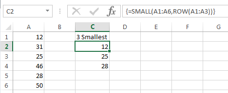
Let’s take this example below where the formula in column C is a multi-cell array formula that is returning the 3 smallest values from cells A1:A6:

The SMALL formula evaluates like so:

=SMALL(A1:A6,ROW(A1:A3))

=SMALL({12;31;25;46;28;50},{1;2;3})

In this case ROW is returning a series of sequential numbers from 1 to 3 and as a result cell C2 returns the smallest value, cell C3 returns the second smallest and cell C4 returns the third smallest.

Problems arise when people try to edit formulas like this that they’ve copied them from somewhere, maybe another workbook, or somewhere they’ve found in a Google search.

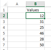
Excel experience tells us to adjust range references to suit our data, so let’s say your data is in cells B2:B7 like so:

You might be tempted to copy the formula above and edit it to suit your data like this:

=SMALL(B2:B7,ROW(B2:B4))

After all, if you're changing A1:A6 to B2:B7 for SMALL shouldn't you also change A1:A3 to B2:B4 for ROW? NO. If you do you'll end up with this:

=SMALL({12;31;25;46;28;50},{2;3;4})

Which would be correct for the values in cells B2:B7 but not for the ROW function reference, which as you can see above now incorrectly returns 2, 3, 4.

The correct formula is:

=SMALL(B2:B7,ROW(B1:B3))

=SMALL({12;31;25;46;28;50},{1;2;3})

Because we want the 3 smallest values, not the 2^nd, 3^rd and 4^th smallest.

So, now you know why ROW, ROWS, COLUMN and COLUMN are typically used you’ll be able to use them in your own formulas and not get caught out editing formulas that already use these clever functions.

Caution

Pay particular attention to how these functions adjust when rows or columns are inserted above (or to the left for COLUMN/COLUMNS), or in between cells containing these formulas as it can yield unexpected results (read; formula errors).

Absolute referencing is your ally but the approach differs depending on whether you're using these functions in an array formula or a regular formula.

Here are some tips; the formulas below will adjust as a result of rows/columns being inserted above/to the left but they will still return the same results:

Regular Formulas

=ROWS($A$1:A1) or =ROWS($1:1)

=COLUMNS($A$1:A1) or =COLUMNS($A:A)

Copy and paste (or fill) the above formulas to extend the range.

Array Formulas

=ROW(A1:A10)-ROW(A1)+1

=COLUMN(A1:J1)-COLUMN(A1)+1

The above formulas will return the numbers 1 to 10. Adjust the range referenced to suit your needs.

Examples of Formulas that use ROW(S) or COLUMN(S) Functions

VLOOKUP with dynamic column index

Summarise monthly data into quarters

Lookup and return multiple matches

List missing numbers in a sequence

Find a column containing a specific value

Remove blank cells from a range