Slicers are a great tool for incorporating interactivity into your reports but we don’t always want to analyse our data with PivotTables and PivotCharts. Nor is our data always in the perfect format for PivotTables.
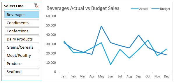
So, let’s look at how we can use the Excel Slicer Selection in formulas which will enable us to create interactive reports that use regular charts with Slicers, like the one below:
Note: Slicers are available in Excel 2010 onwards.
Download the Workbook
Enter your email address below to download the sample workbook.
The Data
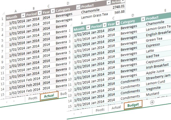
For this example my data is spread over two sheets, each in an Excel Table. The Tables have Names; Actual and Budget. You’ll see these names in the Structured References in my formula later.
Insert a Quasi PivotTable
Since Slicers are connected to PivotTables the first step is to insert what I call a quasi PivotTable, which I've linked to my "Actual" data Table. This is a PivotTable that only has row labels for the items I want displayed in my Slicer.
For example, I want a Slicer for my Category field so I’ve created this quasi PivotTable in cells L4:L12:
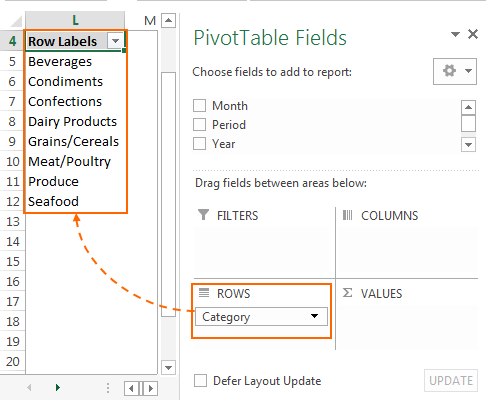
Notice how it has no Values field, only the Category field in the Rows area.
Tip: You can put the field in the columns or filters area instead. It doesn’t really matter. I like to use the Rows area so that if multiple items are selected in the Slicer then they will fill down a column as opposed to across a row, or displaying the text ‘Multiple Items’ in the Filters area.
Insert a Slicer
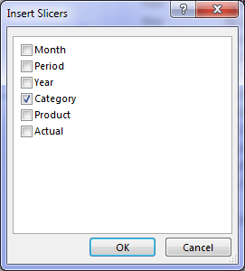
Next I need to insert a Slicer for the PivotTable Category field.
It’s dead easy; with a cell selected in your PivotTable go to the Insert tab > Slicer. In the dialog box (image below), select the field you want to insert a Slicer for:
Note: if you already have a Slicer inserted, you can connect it to the quasi PivotTable by right-clicking the Slicer > Connections > check the box for the quasi PivotTable.
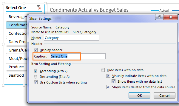
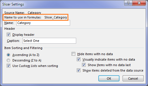
I’ll also change my Slicer caption to say "Select One" to give some guidance to the user. To modify the caption: right-click the Slicer > Slicer Settings, type in a new caption and click OK:
Tip: The reason I only want one item selected in the Slicer is because I’m going to use the SUMIFS function to summarise my data and I’ll be using the selection in the Slicer as one of the criteria. Remember, SUMIFS treats each criteria as AND, so it cannot handle more than one category. For that you would have to use the SUMPRODUCT Function.
When you select an item in the Slicer the row labels are filtered to only display the selected item(s), which can be seen in cell L5 below:
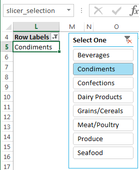
You can see in the name box in the image above that I’ve given cell L5 the Name "slicer_selection", which I will use in my SUMIFS formula.
Use Excel Slicer Selection in Formulas
The table that feeds my chart is in cells H4:J16:

The SUMIFS formula in cell I5 is:
=SUMIFS(Actual[Actual],Actual[Category],slicer_selection, Actual[Month],">="&Report!H5, Actual[Month],"<="&EOMONTH(H5,0))
Notice how the third argument references “slicer_selection” which is the name I gave cell L5. It’s as simple as that, I’m just referencing the row label in the PivotTable that displays the item selected in the Slicer. The SUMIFS formula automatically updates to reflect any changes in the Slicer selection.
Here is the English translation for my SUMIFS formula:
SUM the Actual column of the Actual Table IF the Category in the Actual Table Category column is the same as the Category in the slicer_selection cell, AND the date in the Month column of the Actual Table is greater than or equal to the date in cell H5, AND the date in the Month column of the Actual Table is less than or equal to the end of the month (EOMONTH) date in cell H5.
The limitation is that SUMIFS can only handle one selection in the Slicer. If more than one item is selected then only the first item is reflected in the chart.
Dynamic Chart Label – The Icing on Top
Notice how the title in my chart reflects the selection in the Slicer?
I’ve linked my chart title to an IF formula in cell N4:
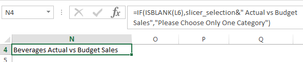
It picks up the Category selected in the Slicer from the PivotTable cell L5 called "slicer_selection" and concatenates the text “Actual vs Budget Sales”, and if more than one Category has been selected it displays this message in the chart title:
“Please Choose Only One Category”
Benefits of Using Slicer Selection in Formulas
Obviously Slicers were designed to work with PivotTables and PivotCharts, and if you have Excel 2013 onwards then you can also use Slicers with Excel Tables.
However, with this workaround we can use Slicers in formulas thus enabling us to summarise data spread over two or more tables of data, which would otherwise require Power Pivot and or Power Query.
This method also enables us to use regular charts which are more flexible than PivotCharts.
Final word: In the Slicer settings you may have noticed a "name to use in formulas" (see image below). This is only for use with Power Pivot models and requires the CUBERANKEDMEMBER function or VBA, but that’s a post for another day.


Hello Mynda. This article helped me a lot in making a simple filter for dashboards. In the beginning of this article, you had mentioned that you did not cover the multi-select of slicers, and that we need to make use of SUMPRODUCT function. Can you please demonstrate how to do so? If already posted as an article, would be of great help if you provided a link to the article.
Also followed you in LinkedIn
Hi Mujeebur,
You can use the SUMPRODUCT function with OR criteria to sum multiple items. You can also use the FILTER function, which would be better if you have a version of Excel that supports it.
Mynda
Hi,
I’m working with membership data in a table and have a column with a range of years, from 0 to 70 yrs, for volunteers.
I’d like to group the years in increments of 10 :. 0 to 9, 10 to 19 etc. to be able to easily track (notice) how many volunteers are approaching milestone anniversaries – 10 yrs increment :. 10, 20, 30, 40, 50, 60, 70
Is there a way to make this work with a slicer getting the data from a table (Pivot Table?
Hi John,
Add a column to your source data that stores the group for each volunteer. Then you can use that field in your PivotTable and Slicer.
Mynda
Hi Mynda,
Thank you for a very useful tutorial. I have one comment – it would be helpful to add an explanation for people who already have reports with a pivot table and slicers on how to attach these to the new quasi-pivot table (the step where you change the existing slicer’s pivot table connections to add the new quasi one).
I’ve looked up this tutorial a number of times – each time i’m either creating a new report or improving an old one, and each time I’ve spent a while trying to remember how I’ve done it last time 😉
Cheers,
Kat
Good idea, Kat. I’ve added a note 🙂
Can this be used in a custom print header?
Hi Bill,
Almost any problem has at least one solution, most of the times imagination is the only limit.
The short answer is yes, but based on your description, I cannot describe a solution, there are many details missing to understand your process.
If you need assistance, prepare a detailed description of what you want to achieve, prepare a sample file, and upload it to our forum, we will help you.
Regards,
Catalin
Nice article. I hadn’t seen it until Ingeborg Hawighorst referred to it.
I will now add the technique to my armoury!
Being me and never knowing when enough is enough, I modified your workbook to accept multiple categories. I first produced an array of results but chose to sum them for the chart.
🙂 thanks, Peter.
I have a table with Sales and Purchase amounts and 2 slicers. One slicer to pick the Department in the Store and the other slicer to pick the year/Qtr. I need to accumulate the sale amount in another column. I also need to calculate the Margin. Do you know how to deal with the moving rows?
Hi Angela,
It’s possible to do these calculations inside the PivotTable, but I’m not sure what you mean by ‘moving rows’. Can you please post your question and sample Excel file on our forum so we can see what you’re trying to do?
Mynda
Maybe I’m missing something, but it seems that the addition of the line-chart, and the subsequent ability to use the Slicer to adjust the view of the line-chart, is missing in the above tutorial. I have simple data, with a list of regions and percentages for several months. You seem to move from the slicer selection formula, right to the dynamic chart label.
I’ve created the slicer/pivot, but at this point, I don’t need a sum, I simply want the line chart to display data based on what Slicer button is selected.
Hi Marie,
This tutorial is about using the Slicer selection in a formula, as opposed to how to create charts and Slicers, so I agree it’s not going to be much help to your scenario.
When you say ‘I want the line chart to display data based on what Slicer button is selected’ this is exactly what the Slicer should do automatically. If your Slicer isn’t controlling your chart then it sounds like the Slicer isn’t connected to the PivotTable that feeds your chart. Try right-clicking the Slicer > Slicer or Report Connections > check that the PivotTable for the chart is selected in the list.
If that’s not it, please post your question and Excel file in our forum where we can troubleshoot further for you.
Mynda
Hi,
Great tutorial, which will help me solve my excel issues. It will help me huge, when the missing graphics will be shown. Are you maby able to fix them?
Thanks Ron.
Sorry about the images, should be all displaying now.
Interesting! How do you handle it when you don’t pick any category but your filter is cleared out (All)?
Thank you!
Hi Di,
That’s similar to selecting multiple items in the Slicer i.e. more than one item is selected and the SUMIFS formula can’t handle multiple criteria for the same criteria range.
In that case you can use the SUMPRODUCT function with an OR operator between each criteria to accommodate multiple items selected, or if you just want to handle one selection or no selections, then you could wrap your SUMIF/S in an IF function that checks to see if there are no selections made, in which case it would just SUM the range, otherwise use SUMIF/S to accommodate the selection in the Slicer.
If you have a lot of items in your Slicer then trying to accommodate every option will make for a very long SUMPRODUCT formula. In that case you might be better off trying to work with PivotCharts, or build a dynamic named range that references the PivotTable range and use that as your chart source range for a regular chart.
Mynda
This is great, Mynda, thanks!
How do you manage to get the chart to change smoothly?
Cheers,
Marcos
Hi Marcos,
That’s a built in feature available in Excel 2013 onwards.
Mynda
I can now understand how to use this useful tool. After converting one of my reports that consists of 20 different tabs based on inventories down to 3 tabs I was very happy. However, I emailed the report out to all the recipients, come to find that Slicers are not usable on smartphones. I open the spreadsheet on my Android and get the message:
“Slicers aren’t fully displayed or interactive. If you data was previously filtered, it’s shown in its filtered state.”
Is there any way to use spreadsheets with slicers on smartphones?
L.E.: We are using Excel 2010 to create the files.
Thanks
Jeff
Hi Jeff,
Even if the slicers are created with Excel 2010, to view them and use them you have to use Excel 2010 or higher versions, or with Excel Online.
You can upload them on OneDrive, and view them with a browser, with Excel Online, instead of using the software installed on your smartphone.
Catalin
It will depend on your phone. On my phone opening a file containing Slicers in Excel Online in Firefox doesn’t display the Slicer at all 🙁 My phone is quite old though!
Mine still has keyboard, it’s not smart 🙂 , I cannot test on it…
😀 now I don’t feel so bad about having a 4 year old phone!
Nice tutorial,I will appreciate if you can share with me the video tutorials.
Thanks
Glad you liked it, Godfred.
There’s no video for this tutorial.
Mynda
Mynda, thank you for the very interesting post. I hope to implement the slicer instead of using a dropdown. It is possible to use the slicer selection to automatically expand when more data is added to the table? For example, if I created the original slicer to select Year when the table currently had data for the years 2010 to 2015. Now that I am adding 2016 data, could “2016” be automatically added to the slicer selections? Or would the original pivot table of Years first have to be refreshed?
Hi Ken,
You have to refresh the PivotTable for the Slicer to pick up the new year, but then you’d want to refresh the PivotTable if you added new data to the source anyway.
You can set the PivotTable to automatically refresh upon opening of the workbook, or with some VBA you can set the PivotTable to refresh upon change of worksheet selection which I teach in my Excel Dashboard course.
Kind regards,
Mynda
Could you create more the option to choose multiple category? For example I want to show the chart which compare actual vs budget for 02 products.Or show the chart of top 3 actual vs budget
Hi Dien,
It’d be easier to consolidate the data with Power Query or Power Pivot and insert a Pivot Chart than try and write a formula to handle a variable number of items selected in the Slicer.
Mynda
I have a PT on which I have multiple slicers that can be applied so would the Power Pivot be a better option in order to ensure that the unsliced total of the PT (when slicers are applied) always equals the total of the source data?
Thanks
Hi Michael,
Power Pivot would be the only way to do this.
Mynda
Great post – very creative! I tried this with a slicer on the table and don’t believe this works. When a table is sliced, it filters the list and the data stays in its original cell, so naming the first cell in the table list does not return the desired result.
Good point, Paula. We could probably write a formula to extract the visible cell, but it’s easier just to use the PivotTable method.
Excellent Artcle.
Thanks, glad you liked it 🙂
Phil
Brilliant and very useful in a lot of situations. Thank you
Thanks, Anika. Glad you’ll be able to make use of it.
Mynda
This is something that will help me tremendously! One question though, what if my data is not broken down by month but rather by day?
Hi Ellen,
I’m glad you’ll find this useful. My SUMIFS formula assumes the data is broken down by day. I just happen to only have one day date for every month.
Mynda