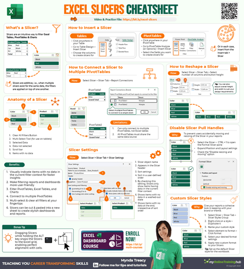
Excel Slicers are a professional way to enable users to easily and intuitively interact with your reports, filtering data in PivotTables, Pivot Charts, Excel Tables and CUBE functions. They're available in Excel 2010 onwards for PivotTables, and for Excel Tables from Excel 2013. In this comprehensive tutorial I cover EVERYTHING you need to know about Excel Slicers.
Table of Contents
1. What are Excel Slicers? 2. Inserting Slicers 3. Using Slicers 4. Formatting Slicers 5. Custom Slicer Styles 6. Copy and Modify Slicers 7. Connect Slicers to Multiple PivotTables 8. PivotTables not Listed in Report ConnectionsWatch the Excel Slicers Video

Download the Workbook and Cheat Sheet
Enter your email address below to download the sample workbook and cheat sheet.

Download the Slicers Cheat Sheet
What are Excel Slicers?
Now I know you can already filter using the PivotTable or Excel Table filter tools, but Slicers are better for two reasons:
- They can control the filtering of multiple PivotTables/Charts (but only one Table)
- They look professional and are more intuitive to use
Have a go yourself using the interactive workbook below.
Warning: don’t go silly and choose too many areas though, or the PivotChart might implode….. what am I thinking? That’s like a red rag to a bull, of course you’re going to try it now that I mention it but at least I warned you!
Data used in chart above is from Greater London Authority (Microsoft Azure Marketplace).
Pretty cool, eh? I'm sure you're now itching to get started with your own Slicers, so here's how:
Inserting Excel Slicers
To insert a Slicer first select a cell in the Table or PivotTable that you want the Slicer to control > then on the Insert tab of the ribbon > in the Filters group you’ll find the Slicer icon.
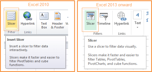
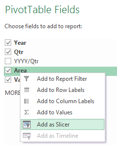
Tip: In Excel 2013 onward you can also right-click on the Field in the PivotTable Field List and choose ‘Add as Slicer’:
Using Excel Slicers
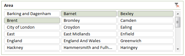
Slicers are intuitive to use, and they allow us to easily filter one or multiple items:
- Click one item to apply the filter for that area
- Click and drag through items to select more than one, or
- Click the first item > hold down SHIFT and click on the last item in your range
- Hold CTRL while clicking to select non-contiguous items
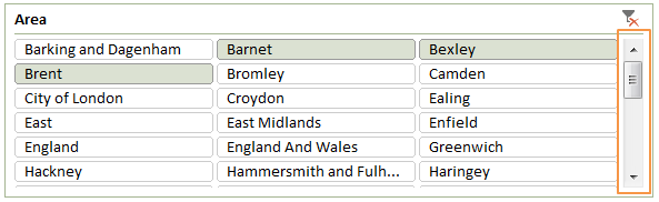
The Slicer displays the selected items in a different colour giving a visual indicator to the user:
And to remove all filters simply click the red x at the top right of the Slicer.
Formatting Slicers
One of the gripes I had with Slicers in the early days was that they were a bit chunky. Since then, I’ve found some of the formatting tricks hidden deep down in the menus that allow you to make them a more manageable size.
I’ll take you through the obvious ones first and then I’ll show you the secret ones 😉
Excel Slicer Settings
Select the outer edge of the Slicer to reveal the Slicer Tools; Options menu. Here we can access the Slicer Settings (Tip: you can also right-click the Slicer to access the Settings):
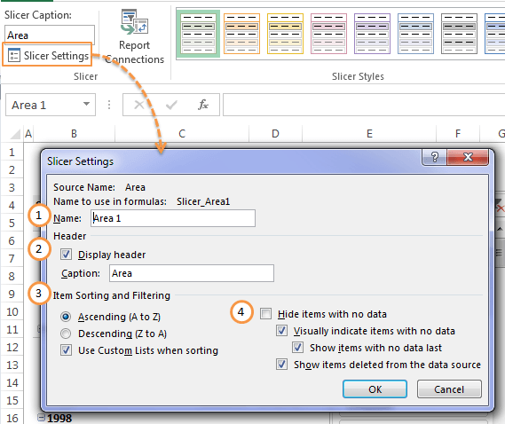
- Change the Slicer name
- Turn the Slicer header off/on, or give it a different caption
- Choose how to sort the Slicer
- Choose how the Slicer should handle items with no data. Note: in Excel 2010 you don't have the option to 'Hide items with no data'.
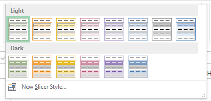
Excel Slicer Styles
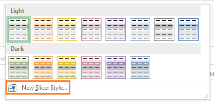
In the Slicer Styles group we can choose the colour and style, or create a new style (note: the colour options will be based on the Theme/Colors you have selected for the workbook in the Page Layout tab of the ribbon, mine is ‘Paper’):
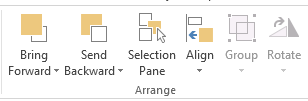
Arrange Slicers
The Arrange group of tools allow you to quickly align your Slicers or move them behind or in front of other objects like charts, shapes, images etc.:
Buttons and Size
The last groups are Buttons and Size; here you can change the number of columns, button height and width and the overall size of the slicer (Tip: you can also use the pull handles which are available when you click the outer edge of the Slicer to change its overall size):
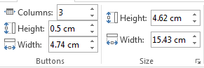
I generally find anything smaller than 0.5cm for the button height is as small as you can go.
If the overall height of your Slicer is too small to display all of the values a scroll bar will be inserted:
Now, while all of the above formatting options are great, they still only allow you to make your Slicer a bit smaller and it’s usually not enough, especially in dashboard reports where spreadsheet Real Estate is at a premium. That’s where the ‘Secret’ formatting options are essential…. Ok, they’re not really secret but they’re not obvious either.
Custom Excel Slicer Styles
One option is to create your own Slicer Style. You can create a style from scratch on the Slicer Tools: Options tab > in the Slicer Styles group click on the down arrow to expand the gallery > click New Slicer Style:
This will open the ‘New Slicer Style’ dialog box where you can format each of the 10 Slicer elements exactly as you want:
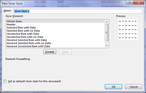
You can even check the ‘Set as default slicer style for this document’ box and use it over and over again, but wait right there because I have a quicker way.
Copy and Modify Excel Slicers
I prefer to copy a Slicer that has the colours I want to use, and then I can just modify the font size and get rid of the border to make it even smaller. To copy a style right-click the style in the gallery > Duplicate.
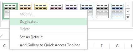
This will open the Modify Slicer Style dialog box:
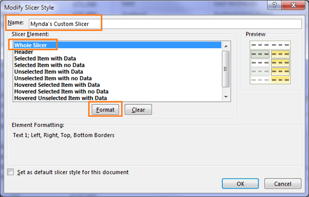
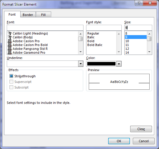
Here you can give it a new name, then from the Slicer Elements list select ‘Whole Slicer’ and click on Format > in the ‘Font’ tab change the font size; I like 9, but it will depend on the font you choose:
Then go to the Border tab and remove the border:
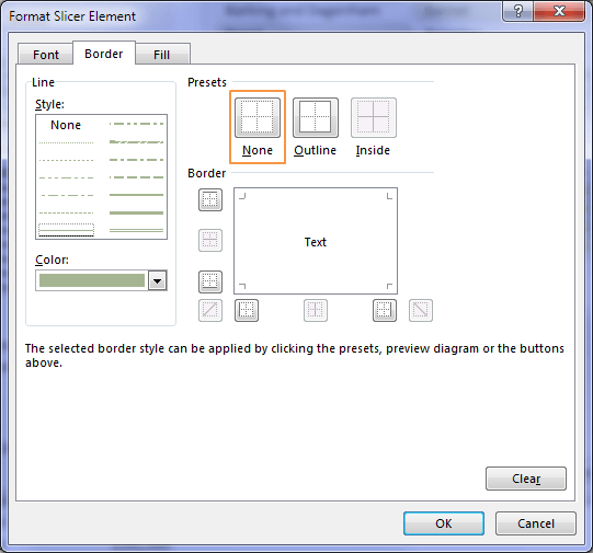
Note: While removing the border serves to make the Slicer appear smaller it is actually still the same size. However, now you can squeeze it into a smaller space by placing the edges of the Slicer underneath other objects, like charts, without it being noticeable.
After duplicating your Slicer style you then need to apply it to your Slicers. If you have multiple Slicers, you can select them all (hold down SHIFT while you select each one), then click on your new style in the Slicer Style gallery.
Ok, now that your Slicer is more compact, you’ll be able to squeeze it into your report.
If you want more customisation, check out this dedicated tutorial on Excel Slicer formatting for further tips on how to tweak them to your liking.
Connecting Excel Slicers to Multiple PivotTables/Charts
Once you’ve inserted your Slicer you can go about choosing which PivotTables/Charts you want it to control.
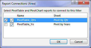
To do this; right-click the Slicer and choose Report Connections. This will open the dialog box below and you can check the box for the PivotTables you want the Slicer to control:
PivotTable not Listed in Slicer Report Connections Area
An Excel Slicer can only control PivotTables which share the same Pivot Cache. Typically, PivotTables which reference the same data source share a Pivot Cache, but not always. If the PivotTables you want to connect to don't appear in the list, then you'll know the cause is separate Pivot Caches
The easiest way to fix PivotTables that aren't appearing in the Slicer Report Connections area is to copy one of the PivotTables that is in the list, and modify it to replicate the missing PivotTable. This way you'll ensure the PivotTable is sharing the same Pivot Cache.
Note: If you copy a PivotTable that is already connected to one or more Slicers, the copied PivotTable will also be connected to those Slicers, so you may need to edit the Slicer Report Connections.


Hi Mynda,
Is it possible to create an excel slicer and limit the number of slicer options to say 5. For example if there are 20 countries and you want the slicer to show only 5.
Hi George,
You can add a new column, with a formula to set the Country names as “Other”, if that country is not in the list of 5 you need, use the new column as a slicer.
Hi Mynda!
You are the best by far at explaining Excel.
I have seen numerous tutorials but your work is outstanding.
Keep it up!
Greetings from Mexico!
Thanks so much, Daniel!
Hello,
love you lectures, could not download the working file, link might not working.
Thank you very much!
Thanks for letting us know, Aleks. I’ve fixed it now.
Hello
I always find your tutorials so helpful.
I am having a nightmare time with a pivotable profit and loss I set up. The slicers are not interacting with each other as they should. I have 3 layers (3 slicers) – Region, Location and then DC so theoretically you should be able to select the Region which should then show you on the Location slicer which locations are in that Region and then select a Location which then shows you on the DC slicer which DC’s are in the Location.
I have created a similar pivot table before and the slicers work as expected but I cannot for the life of me get them to work on this pivotable profit and loss which I have invested a lot of time into.
Any suggestions why the slicers wont work?
Hi Laura,
Please post your question on our Excel forum where you can also upload a sample file and we can help you further. If necessary, anonmyise the data before sharing your file on the forum.
Mynda
Hello Mynda,
Please help me this case: I have data like:
Item Sales Jan Pur-Jan Inv-Jan Sales-Feb Pur-Feb Inv-Feb
Hat 5 7 2 4 8 6
Shoes 3 8 5 2 3 6
Is there any way I can add slicer to choose to view Sales – Purchase – Inventory?
Ted
Hi Ted,
Not with your data structured like that. You need to put it in a tabular layout so you can build a PivotTable and use Slicers. You can use Power Query to unpivot the data.
Mynda
Hi Mynda,
Sorry to not explain clearly.
You indicated om tabular layout rule: “Each Column contains a type of data e.g. date, order number, quantity, amount, salesperson, region etc.”
My data column is Sale-Jan, Inv-Jan, Sale-Feb, Inv-Feb and so on. so they are different type of data.
My data row is Shoes, hat, etc
So in Pivot table, I want to see things by months. For example, I choose hat & sale, so pivot will indicate sale of hat by months. However, I need to choose Sale-Jan, Sale-Feb; not choose Jan only. Inv will be the same, I need to choose Jan-Inv, Feb-Inv. This will be problem if I have 15 months, mean I need to untick 15 months of Sale and tick 15 months of Inv if I want to switch.
It is difficult to explain with words and my English. If you are not clear, please let me know your email. I will send an example
Regards,
Ted
Hi Ted,
Can you please upload a sample file on our forum? Will be much easier to help you on your specific data structure.
Create a new topic after sign-up and upload your sample.
See you there
Regards,
Catalin
I cannot work out nor find how to set a slicer to work on a count field in my pivot table.
I have tried filtering pivot table data but not permitted, and count field is not an option for inserting slicer.
I have a list of companies, a count distinct column and a count column.
The count distinct tells me how many companies have downloaded my docs, and the count column tells me how many times that have downloaded the docs. (The docs change). I also have max and min date for each company so can see when they downloaded/most recently downloaded etc.
I want to only see companies that have downloaded once (ie filter out/not display companies with more than 1 in the count colum.
Thanks
David
Hi David,
If you just want to filter for counts > 1 then you should use the filter buttons on the PivotTable to do this. It’s not a job for a Slicer. Hope that points you in the right direction.
Mynda
hi, I would like to change a slicer which is in horizontal to vertical
Hi Benert,
Simply change the number of columns to 1 on the Slicer tab of the ribbon.
Mynda
You’re a real G for doing this. I’m in tears. Thank you Mynda. We stan an excel queen.
🙂 Glad you found it helpful, Dan!
I’m still using Excel 2007. How do I solve the Slicer problem?
You need to use form controls and VBA to create a similar effect to Slicers. I cover this in my Excel Dashboard course.
Mynda
Yesterday morning I awoke to all the Power Pivot dashboards I built for my company having all slicers contain a red x in the upper right hand corner REGARDLESS of whether or not the slicer was actually filtered. It’s like being in a plane with all instruments are giving off warnings regardless of the actual situation. This is literally an unmitigated disaster as all dashboards are much harder to understand now. Scrambling to find a fix to what is by an order of magnitude the most shocking and disastrous bug I’ve ever encountered. I’ve contacted the Excel development team but this is requires and urgent fix. I’ve found that others have recently encountered this as well but with no fix. Does anyone have any idea how to fix this?
Hi Steve,
I’m not aware of this bug. You didn’t say what version of Excel you’re using so it’s difficult for me to investigate further or escalate with Microsoft.
Mynda
Thank You Treacy & Team. I am surely learning !
Is there a convenient way to set a slicer to “Size but don’t move with cells”? Not having this feature has plagued my dashboards for years.
Hi Steve,
Usually, you have more than 1 slicer, all you have to do is to select them all, then right click and choose Group.
This way, all will be a part of the same group, and you can set that group properties to not move or size with cells.
Hi there,
This is absolutely incredible!! Best site I’ve seen – ever!!! A good idea would be to add this training to an app?! Apologies if I’ve missed this of its already available.
This has helped me so much. I’ll def be sharing.
Thank you so much!
Gem (Belfast, NI)
Thanks for your kind words, Gem 🙂 Glad we can help.
Hi Mynda,
Could you please clarify me my problem.
I have created a pivot table where the column field includes sum of Jan, Feb, Mar and so on. I want to filter as only Jan, feb or any other month. I could have done it if I have created from column labels but I have nothing in columns, everything in values field. How can I use slicers in this case to filter my datas.
Without seeing your layout, my guess is that you have sales values with column headers like Jan, Feb and so on. You should reformat the data to have all the headers in a column, this column will contain all months: Jan, Feb, then next column should have the corresponding amounts.
You can upload a sample file on our forum (create a new topic after sign-up), if you need help, if you’re not used to using power query to reformat data.
Excellent tutorial, can’t believe it’s free. Thank you. I will be recommending it.
Thanks, Linda! Glad you found it useful.
First, thank you for your email with all the professional training material. You rock!!!
Is it possible that we can download your web training material in PDF?
Why I ask is that I have to print your training material from your email / website, then scan it, so I can have an electronic copy on my laptop. This results in wasted paper and additional time to have an electronic copy on my computer.
Hi Sean,
Glad to hear you like it.
You can simply print the web page to PDF. If you don’t have a PDF printer, you can install it, there are lots of PDF printers for free: PDFCreator, DoPDF, and so on.
Hi Sean,
I’m actually looking at a way to do this. I’ll keep you posted about this. Hopefully will get something to yo in the next day or two.
Regards
Phil
Nice. Can’t wait to try
Hello Mynda – I love your training courses and website! And I love the slicers – they are wonderful tools but I have an issue that comes up every now and then that I can’t figure out.
Sometimes, the slicer will not remove the buttons that “contain no data” when I select “Hide items that contain no data” in the Slicer Settings. Can you please help me out – what am I missing? Thanks
Hi Brandon,
Great to hear you’ve embraced Slicers.
The answer to your question is, it’s easily fixed by right-clicking the Slicer > Slicer Settings > uncheck ‘show items deleted from the data source’. If your version of Excel doesn’t have this option then you can right-click the PivotTable > Options > Data tab > set ‘Number of items to retain per field’ to None.
Mynda
Hi Mynda,
Thank you so much for all the valuable Excel information you provide in an easy to understand manner.
I’ve created a slicer for my dashboard which includes 3 years of data. The charts display a different color for each year. Is there a way to coordinate the color displayed on the chart with the corresponding Year slicer button?
Hi Marie,
Thanks for your kind words. Glad we’ve been able to help 🙂
You can’t set Slicer buttons different colours within the same Slicer so this wouldn’t work for the different years, sorry.
Mynda
Hi Mynda,
The interactive workbook at the top of the Slicers Tutorial is blank with a “The Connection Was Reset” message where the workbook should be.
Is there some way this can be fixed? It would help a lot in understanding the Tutorial to be able to see the workbook.
Thanks,
Tom D
Hi Tom,
The interactive workbook is displaying for me. Perhaps you could try again or try a different browser.
Mynda
Hi Mynda,
First of all my compliments to the information you give on this website. For me it is a great source of help. Specially the way you explain things is of great help.
Now my question. I am creating a pivot table and want to use quite a number of slicers . Problem is that they use a lot of space on the worksheet. I was wondering if it is possible to turn them into dropdown lists. I cannot find it as a standard layout option, so I assume I need some kind of trick, if it is possible at all.
Thanks in advance for your answer.
Best Regards,
Johan
Hi Johan,
You can’t collapse Slicers, the best you can do is make the buttons and font in the buttons smaller.
Alternatively you can use a Combo Box (drop down list) and a macro to control multiple PivotTables similarly to how Slicers work. I teach this technique in my Excel Dashboard Course.
Kind regards,
Mynda
I attended the one-hour webinar on Pivot Tables with Slicers and learned so much! I created an informative dashboard for our 5-year budget prep and it has been a great hit! I want to put them everywhere now!
That’s wonderful, Valerie 🙂 I’m glad you found it so useful.
Happy dashboarding!
Mynda
I loved slicers on pivot tables in Excel 2010 but slicers on tables in Excel 2013 are flipping awesome! I maintain some metrics for one of our managers. He wants to track a 13-month rolling time period. I was using pivot tables and regular tables to collate the info and each month had to go in and manually adjust 7 different charts. I dreaded working on that file.
Enter Excel 2013. I did a complete renovation of my tables. I combine formulas to minimize the number of tables I needed, lined the 7 tables with charts up left to right, and inserted a slicer on the first table. Excel only charts what it can see so when I select the months in the slicer, all of my tables change. After I paste in my raw data, two clicks and all of my charts are updated. Sweet!!
Niiiiice! Very nice. 🙂
So this does not work for an Excel Table. Is there a Options setting that needs to be changed?
Hi TC,
Slicers only work with PivotTables in Excel 2010. In Excel 2013 they also work with Tables.
Kind regards,
Mynda
I hope this isn’t a stupid question and I have overlooked the answer. After I have inserted my slicer and selected my fields, I now what to remove a couple fields and add a different one to the slicer. How do I do that?
Hi Wanda,
The items in the slicer are based on your PivotTable source data. If you want new items to appear then they must be present in your source. If you have removed any trace of old items and they’re still in your slicer then you can change the settings:
Right-click – Slicer settings – uncheck the ‘show items deleted from the data source’.
Mynda
Thanks
Thank you very much for the wonderful article. I can now slice and dice my data and produce brilliant dashboards. I have one question though…..Can we connect two pivot tables of different pivot caches with a single slicer?
Kind Regards
Xolani (South Africa)
Hi Xolani,
Great to hear you found this article useful. Unfortunately you can’t control PivotTables with different pivot caches with the one Slicer.
Kind regards,
Mynda
Mynda: These are great formatting tips. I am a new fan .
My question is: Can you remove individual slicer buttons from the list of sliders that are created when you Insert Sliders?
For example, I might base my sliders on the field “Color” which has 20 different possible values (in my case – color of widgets). But I only want certain of these “colors” to show up as slicer buttons. Unfortunately, all 20 buttons are created. I have tried hiding the colors I don’t want to pivot on, by putting a text box in front of them, but this is a very ineloquent solution. I have searched and searched for a solution to be able to delete the unwanted slicer buttons, but so far no luck, Hoping you may provide a work-around to this limitation in slicers.
Thanks in advance…
Hi Michael,
Glad you’re now a Slicer fan 🙂
You can’t choose which buttons to display in your Slicer but you can hide items with no data. So, what you need to do is inset another column in your source data for your Slicer. Let’s call it ‘Slicer Colors’. In this column only enter the colors you want to appear in your Slicer. I’d copy your original color column and then delete the colors you don’t want in your Slicer (just the color name from the cells, not the whole row).
Now refresh your PivotTable and insert a Slicer for this new column. You should have an item called ‘Blank’. Now right click the slicer > Slicer Settings > check the ‘Hide items with no data’ under Item Sorting and Filtering.
Your slicer should now display the colors you want.
I hope that helps. Please let me know if you get stuck.
Kind regards,
Mynda
Hi Mynda,
Is it possible to disconnect a copied slicer to its precedent slicer? As I want an independent pivot table and a slicer for other purpose.
What i did it to create a different cache even though it is basically referring to the same source.
Wondering if there is a more direct way to to so?
Cheers,
Hi MF,
You can just right-click the Slicer and choose ‘Report Connections’ and then deselect the PivotTables you don’t want the Slicer to control. The Slicer must be connected to at least one PivotTable so you can just set up a dummy PivotTable with the Slicer field in the rows or columns area.
I hope that makes sense.
Mynda
Hi Mynda,
Thanks for your super fast response. Appreciate that! 🙂
Sorry that I may not make my point clear.
My problem is: I have many duplicated slicers and they are all connected. Even though I can disconnect the slicer to a pivot table, I cannot disconnect the slicer from the rest of the duplicated slicers. Whenever I select an item on the slicer, the same selection applies to the rest of the duplicated slicers. And I was trying to find a way to get around it. Any idea?
Hope I have made my point clear this time. ;p
Hi MF,
Sorry, I misunderstood. Since you’ve cloned your Slicers you cannot disconnect them as they are part of the same hierarchy. You’ll have to delete the cloned ones and insert new ones, as opposed to copying and pasting them.
Kind regards,
Mynda
Hi Mynda,
Thanks for your advice. I think that’s the way to achieve that for the moment.
Cheers,
MF 🙂
Mynda,
Thanks for the great post. However, when I try to set up two simple pivot tables that have similar headers, I add slicers to one pivot table, right-click to go to Report Connections. The dialog box appears but only contains the PivotTable for the slicer that was created. Any thoughts on why both don’t appear? Thanks,
Thanks, Michael.
Only PivotTables which share the same Pivot cache can be controlled by the one Slicer. So if only one PivotTable appears in the Report Connections it means they have different caches.
Hope that helps.
Kind regards,
Mynda
That was it! Thanks!
Very new to me but useful trick thank you.
Glad you liked it, Ravi 🙂
Excellent!
Any chance of getting a copy of the actual raw data file?
Hi Sam,
You can download it by clicking the Excel icon in the bottom right of the Excel Web App interactive workbook at the top of the post.
Kind regards,
Mynda
Great little trick with pivot. Tried it today at work and absolutely loved it
Thanks, Edwin. Glad you liked it.
Mynda
Way cool! Excellent format and layout ideas. Thanks for sharing.
Thanks, Jef 🙂 Glad you liked it.
Mynda
i did’t find slicer………..m using excel-2007
Hi Vinutha,
Excel 2007 doesn’t have Slicers. Only from Excel 2010 onwards. Sorry.
Mynda
Nice Tweak Mynda. My slicer appears much cleaner without the borders. Is there a way to establish my custom slicer style, in any instance of Excel that I open?
Regards,
Bud in Connecticut USA
Hi Bud,
You can Right click on your Custom Slicer Style, and select Set As Default, that’s all you have to do, but Custom styles are saved at the workbook level. This means that while your custom style is saved and travels with your workbook, any new workbook will not have your styles included. The workaround for this limitation is save your workbook as an Excel template. To do so, choose to save the workbook with your custom slicers as an Excel Template (*.xltx) file. Once you’ve got that saved, you can open your template file to start a new workbook with your custom style included.
Cheers,
Catalin
Precious, precious, precious!
Thank you!
Thanks, Maxime 🙂
Agradezco todos los aportes, aunque no soy bueno en el Inglés he aprendido grandes cosas de Excel que es mi pasión, Especialmente los DASHBOARDS, los cuales espero muy pronto poder aprender a realizarlos.
Saludos desde Colombia.
Gracias,
Gracias, Angel. Es agradable saber que puedo ayudar.
Saludos cordiales,
Mynda