Excel Slicers are great, but they’re a bit on the chunky side and that can be a pain when you’re building reports like Excel Dashboards where space is limited. Unfortunately, the Excel Slicer Formatting available on the Slicer contextual tool tab is limited, as you can see below:
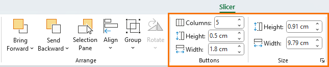
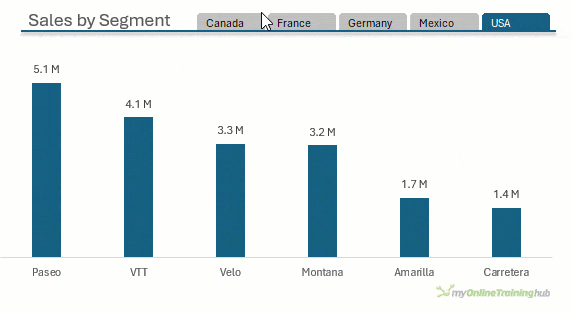
I’m going to show you how we can uncover the settings and make them much smaller, and some tricks like those in the example below to make them look like tabs. Plus, how to prevent users accidently activating the pull handles and resizing them:
Watch the Excel Slicer Formatting video

Download Workbook
Contains step by step written instructions with screenshots that you can use as a reference.
Enter your email address below to download the sample workbook.

Excel Slicer Formatting Step by Step
The trick to making your Slicers small is to create your own custom Slicer style.
Step 1: Select a Slicer to reveal the contextual Slicer tab
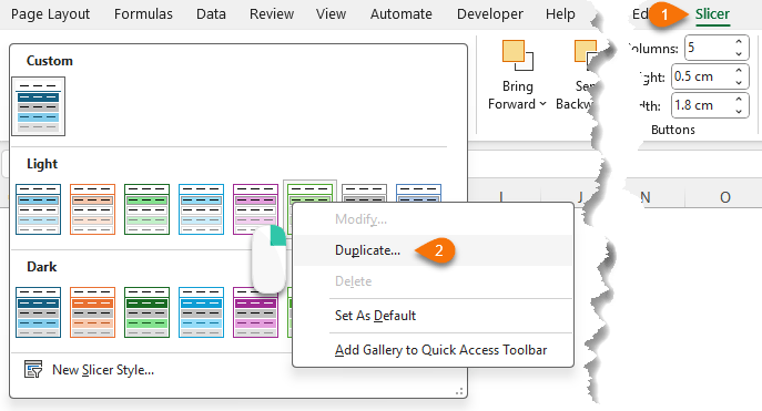
Step 2: In the Slicer Styles gallery choose a style that’s close to what you want. Trust me, this will save you time. Right-click the style you like > Duplicate:
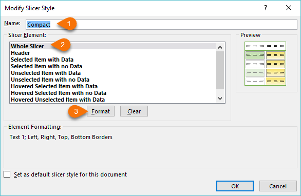
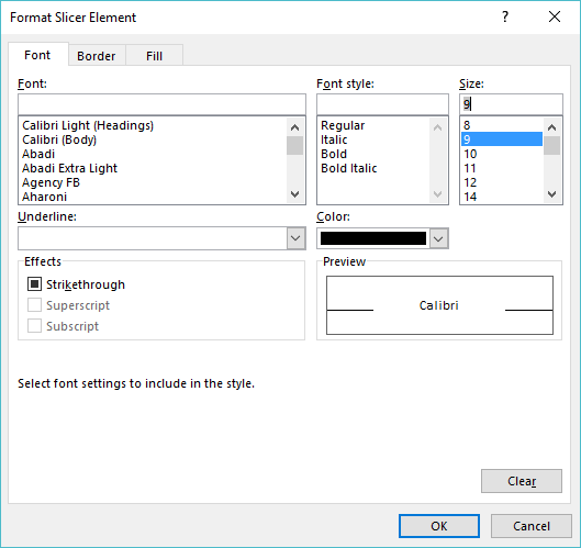
Step 3: In the Modify Slicer Style dialog box that opens, give your style a name. Mine is called ‘Compact’. Then select ‘Whole Slicer’ in the Elements list and click ‘Format’:
Step 4: In the Font tab alter the font size as desired. This will allow you to make the button height smaller.
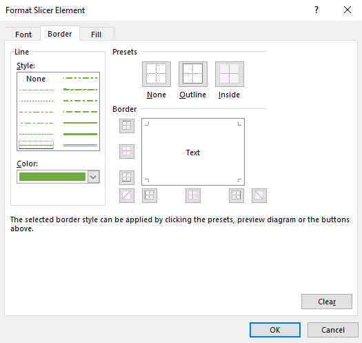
Step 5: Go to the Border tab and set the border to ‘None’. This will enable you to overlap the Slicers slightly, as you won't be constrained by the borders:
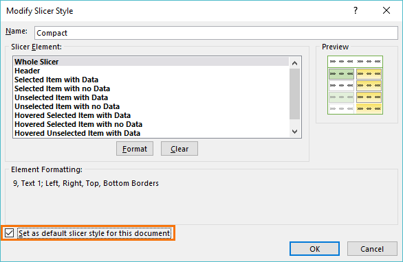
Step 6: After you click OK in the Format dialog box you’ll be taken back to the Modify Slicer Style dialog (image below). You can also select the other elements and modify them as required, but generally I’m too busy for fiddling about with that.
Be sure to check the ‘Set as default slicer style for this document’ box:
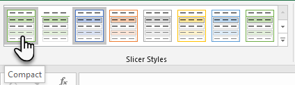
Your Slicer style will be the first in the gallery:
Now all you need to do is apply it to the Slicers already in your workbook. Tip: Select one Slicer and then press CTRL+A to select all the Slicers. Now you can apply the formatting with one click.
Note: Pressing CTRL+A with at least one Slicer selected will select all objects, so if you have images or shapes in the worksheet CTRL+A will also select them.
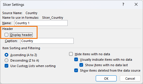
Tip: you can also hide the Slicer header, but this also removes the clear filters 'X' in the top right. You can remove filters by selecting all items in the Slicer, but this may be inconvenient in Slicers with lots of items.
To hide the Slicer header right-click > Slicer Settings:
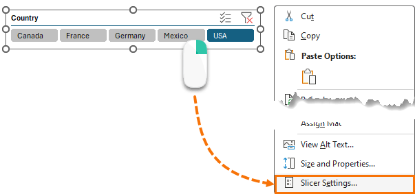
In the Slicer settings dialog box deselect 'Display Header':
Slicer Tabs
Create a tab effect by reducing the height of the Slicer until the bottom of the button is chopped off. In my example it's 0.91 cm high:
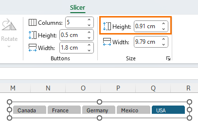
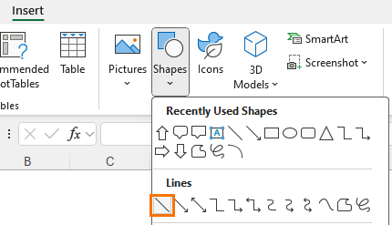
As a finishing touch, draw a line shape under the buttons to give the appearance of the top of a page:
For extra credit, add a drop shadow to the line to make it pop (Shape Format > Shape Effects > Shadow):

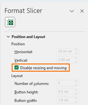
Prevent Moving and Resizing
It's super easy to accidently activate the pull handles when clicking Slicer buttons. Not only do they then look ugly, they can be accidently moved or resized. An easy way to prevent this is by setting the Slicer to 'Disable resizing and moving' in the Slicer Formatting pane:
Items With No Data
When you group dates in PivotTables, you automatically also have items added for dates less than the first date in your dataset and greater than the last date. These show up in the Filter drop downs and Slicers:
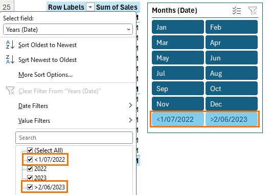
Unfortunately, there's no way to remove these items, but we can hide them from displaying in our Slicers via the settings (right-click):
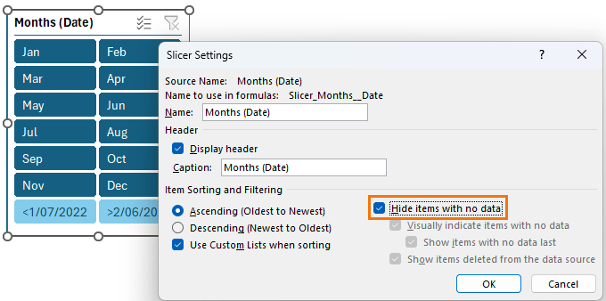
Notice that this also hides items deleted from the data source.
More Excel Slicer Tips
One of the limitations of Slicers is you can’t force people to only select one item, and this important when you’re linking the slicer to a formula that can only reference one item at a time, but I’ve got a clever workaround for this: How to force Slicers to single select.
Slicers are an essential tool for making your reports polished and easy to use. Learn more tips including how to connect them to multiple reports with our comprehensive Excel Slicers tutorial, including video and workbook.
If you'd like to get your PivotTable and Slicer skills up to speed, check out our PivotTable Quick Start course.

How do I hide ‘(blank)’ from displaying on a slicer?
Hi Karin,
Filter the ‘Blanks’ out of your PivotTable and then set the Slicer settings to ‘hide items with no data’.
Mynda
Hi Mynda,
Your tutorials have been tremendously helpful and well put together. I found your site by (happy) accident, and I’ve been able to use your insights in a variety of projects. Thanks for sharing your Excel knowledge and specifically for helping me understand the visualization capabilities that Excel has.
Thanks,
RT
Thanks for taking the time to comment and your kind words, Randy! I’m delighted we’ve been able to help 🙂
Hi Mynda,
Is there a way to have your custom slicer settings to be applied another file (travel across other workbooks)? It doesn’t seems like it.
Thanks,
RM
Hi RM,
You could apply them to your default workbook so that every new file you create has access to them, but I’m not aware of any way to copy them to an existing workbook.
Mynda
I have been using a slicer in my dashboard for some time now, but have discovered that one of the buttons in the slicer is not formatted like the rest. It is white, where all of the other buttons are blue (as they should be). Any thoughts?
Hi Ellen,
Is that slicer’s format a default format? Make sure you have data under that button, usually the buttons with no data are formatted differently.
Very useful tutorial.
I am not being able to hide “blank” buttons from slices that show data from a table. It is possible to do it with pivot table slices. How can I hide the “blank” buttons on table slicers?
I use the MSOffice 365
Thanks.
Hi Wilson,
I’m not aware of any way to hide blanks in Slicers for Tables, sorry.
Mynda
Hi Mynda,
Great tutorial, but I am unable to actually edit the font once at step 4. When the Format Slicer Element dialog comes up, both Font: and Size: have lots of entries, but they are all grayed out. This is the case regardless of which slicer element I attempt to modify (Whole Slicer, Header Row, etc).
I am also unable to modify the font or size in the Timeline control, if this gives any additional hints, while I can alter font & size for the PivotChart itself.
Using Excel 2016 on Mac.
Any thoughts on what is causing this, and if it can be modified?
Hi Xander,
I don’t have a Mac I can test it on, but it sounds like a Mac limitation.
Mynda
Hi Mynda,
Thanks, this is great, however – there is always a “however”
With all of the “selected items” on the slicer, I make the font size “4” and most can be displayed. However, I see no way to reduce the size (width) of the slider bar on the right, which make the slicer look klutzy.
Can this be done?
Thanks,
Ted
USA, Detroit Michigan
Hi Ted,
No, sorry you can’t change the size of the scroll bar.
Mynda
Explicit and useful presentation. Saved my skin!
Glad I could help 🙂
Hi Mynda, this is another great presentation! I have a different question about slicers that I have attempted to find information about… is it possible to limit the names in a slicer to the top 100 (such as I have done in the pivot table itself)?
I have a pivot table with customer names, and I have sorted and filtered so the table only shows the top 100… I also have a pie chart with other data that is linked… I would like the slicer for the pivot table to operate the pie chart (which I know how to do) but I want the slicer to only show the names in the pivot table, all the customers… any thoughts?
John
Hi John,
Many things can be done, but unfortunately there is no easy way to change the values displayed in slicers. Usually the way it works is good enough for most people, and it’s the normal way to go.
There can be only workarounds, like adding a rank column in your source data, and create another column with a formula to return customer name only if the rank is less than 100. You will this column as a slicer, but you will still end up with a blank entry in the list of customer names.
I want to save the new style to use in other workbooks, but when I closed my workbook (saving changes), then opened another workbook with a slicer, my Compact style wasn’t available. How do I save it for any workbook?
Hi Jomili,
The style is workbook specific. You can add it to a template, or your default Excel workbook.
Mynda
Hi Mynda
I use a colour fill as part of the Normal style to conceal/identify cells that do not form part of my spreadsheet model (grid lines are only made visible in the working ranges of the sheet). That immediately exposes the fact that the white format on tables and pivot tables is actually ‘No fill’ which causes extra work formatting those objects.
Much worse though, are slicers which in Office 2010 acquire ugly black backgrounds. In that instance I want the background to be ‘No fill’ to show the sheet colour but, last time I tried, I finished up by defining every aspect of a custom slicer from the bottom up. I did not enjoy the experience!
Any ideas?
Hi Peter,
It looks like a bug in the customisation options for Slicers because you can set it to ‘No fill’, but it still has white fill (as you mentioned), even in Excel 2016/Office 365. However, you can format the fill the same colour as your background and this only has to be applied to the ‘Whole Slicer’ element.
Mynda
Thanks Mynda. That gives hope for when I eventually move from Excel 2010. At present the slicer background shows as black which is hideous. I then turn the Whole Slicer to the palest grey only to have every button, with or without data, selected or not, matching the slicer background perfectly!
Yes, I spend so much time reformatting, rearranging, resizing and overlapping slicers to try to make them take up less space
If the header is to be displayed, I often give it a more meaningful title to help the less Excel-aware users (depending on slicer width, but one extreme example I have used is “Profit Centre(s) – select multiples by dragging, shift-click to extend or control-click to add/delete; click icon on right to reset”)
and as a footnote, I’ll always deselect “Show items deleted from data source” – can’t think why anyone would want this and, even more so, can’t fathom why showing them is the default
Similarly with retaining deleted items in pivots – why? (this has been a huge gotcha with grouping dates, which can’t be done if there ever was a non date and this is checked)
jim
I hear you, Jim!