Splitting data over multiple sheets is perhaps one of the worst Excel crimes I see. It’s a crime because it breaks the rule that source data should be in a tabular format. Tabular data is what we need for PivotTables and many functions like SUMIFS, COUNTIFS, INDEX, VLOOKUP etc.
To have your data in any other format is just going to make your Excel life difficult. Anyhow, that’s enough ranting about data layouts. I do enough of that here.
Thankfully we can easily consolidate Excel sheets with Power Query in just a few clicks of the mouse.
Workbook Download
Enter your email address below to download the sample workbook.
Watch the Video

Power Query Consolidate Excel Sheets
Let’s take the file below that has a separate sheet for each salesperson’s order data (Buxton, Maxwell, Jarvis and Everton), and another sheet containing ‘Other Stuff’ 1:
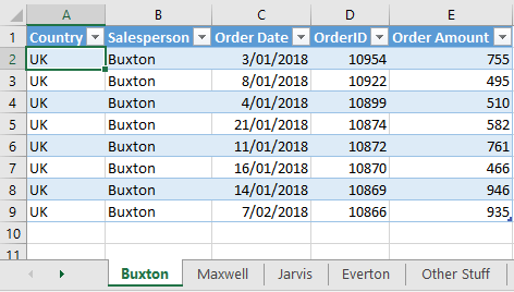
1. The ‘Other Stuff’ sheet simply represents a typical file that has another sheet(s) containing information that isn’t source data2. I included this sheet so that I can address how to handle these sheets when consolidating source data in Power Query.
2. Source Data is data that I want to include in my consolidated data set. It’s the source of your analysis.
Key Points to Using Power Query Consolidate Excel Sheets
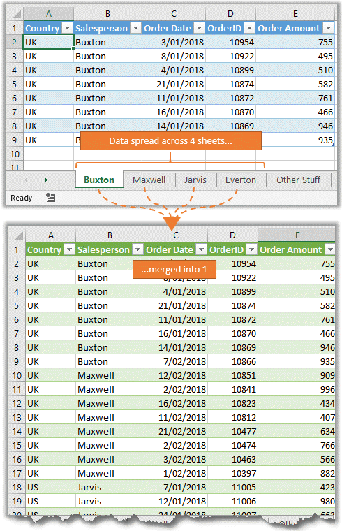
Ideally, we want the source data on the four salesperson’s sheets merged into one sheet because that’s going to allow me to summarise it with a PivotTable or easily analyse it with any of the built in Excel functions, which is not possible when the data is spread across multiple sheets.
The technique I’m going to show you here requires:
- The data on the sheets I want to consolidate are formatted in an Excel Table or has a been given a Named Range. This is required for Power Query to find the data.
- The table structure (column names) on each sheet you want to consolidate are the same.
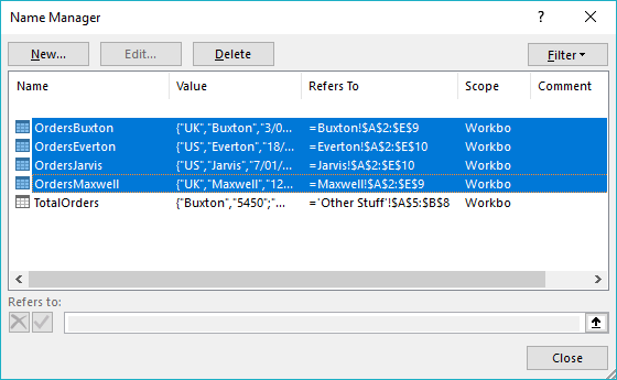
- The name of the Tables or Named Ranges use distinct nomenclature that is different to any tables/ranges you don’t want to include. E.g. my salesperson tables all begin with ‘Orders…’, as you can see in the Name Manager below:

Note: The ‘TotalOrders’ table is on the ‘Other Stuff’ sheet and the name purposely doesn’t begin with ‘Orders’ because it isn't part of my source data. This will allow me to filter the tables and consolidate only those that have names beginning with ‘Orders’.
Consolidating Excel Sheets using Power Query
Ok, now the housekeeping tasks are out of the way, let's look at how we can use Power Query to grab the data off the salesperson sheets and merge it into one table:
Written Instructions
Step 1:
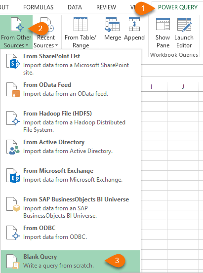
Create a new blank query in the file containing the sheets you want to consolidate. For Excel 2016 or Office 365 take the following steps: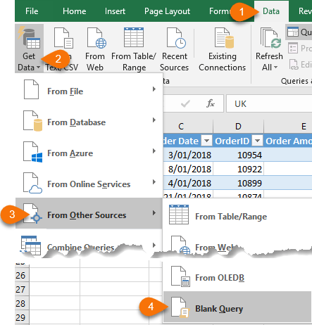
In Excel 2010 or 2013 take the following steps:
Note: If you don’t see the Power Query tab in Excel 2010 or 2013 you can download it here.
This opens the Power Query Editor window.
Step 2:
In the formula bar type:=Excel.CurrentWorkbook()
As shown below:
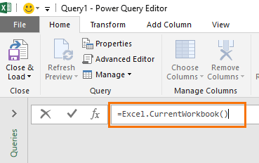
Note: Power Query functions are case sensitive.
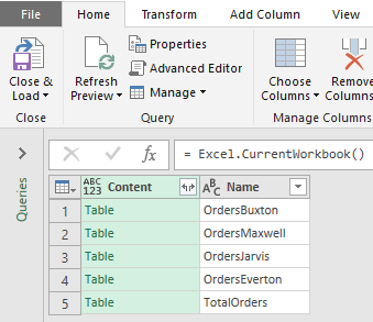
Step 3:
Press ENTER. This returns a list of the Excel Tables, Named Ranges and Filtered Lists in your file:
Step 4:
Filter the ‘Name’ column for items that ‘Begins With…’: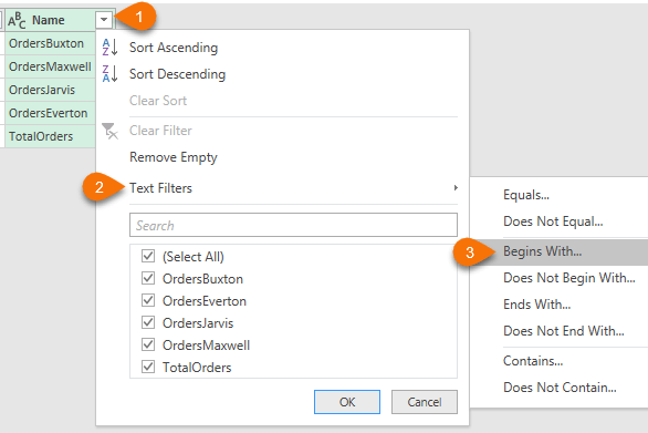
In the ‘begins with’ field enter ‘Orders’:
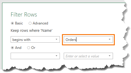
Using a consistent nomenclature allows me to add more ‘Orders…’ tables to my file in future and Power Query will automatically include them upon refresh. Of course, if I’m sure I’ll never add any more sheets that I want to include in the consolidated table then I could simply use the check boxes in the Filter list to select the tables I want.
Step 5:
Now I only have the tables I want to consolidate, I can click the double headed arrow on the ‘content’ column to expand the data:Note: If you don’t deselect ‘Use original column name as prefix’ each column header will be prefixed with ‘Content’. E.g. Content.Country, Content.Salesperson etc.
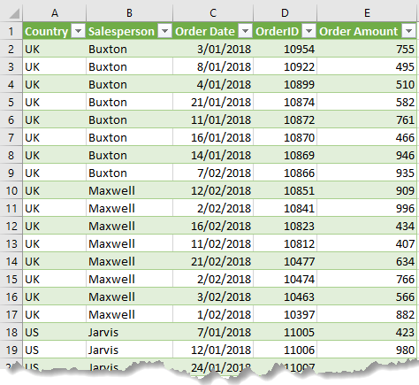
And with that I have my data consolidated into one table:
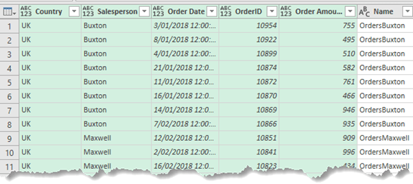
Notice that the last column contains the name of the source Table. You can click on this column header and DELETE it if you don’t want it.
Step 6:
Set the Data Types. It’s important to tell Power Query what type of data you have in each column; dates, text, decimal numbers etc. To do this, click on the icons in the top left of each column and select the data type from the list: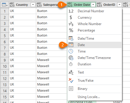
Note: This isn’t formatting, as that’s done in the Excel sheet. These are data types required by Power Pivot (if you’re using it) and will help Excel identify what cell formatting it can automatically apply if any.
Step 7:
We’re almost done. Give your query a name. This name will be inherited by the Excel or Power Pivot Table, so choose carefully avoiding the nomenclature for the tables you are consolidating. i.e. don’t begin with ‘Orders’, otherwise this table will be included in the query and you’ll double count your data!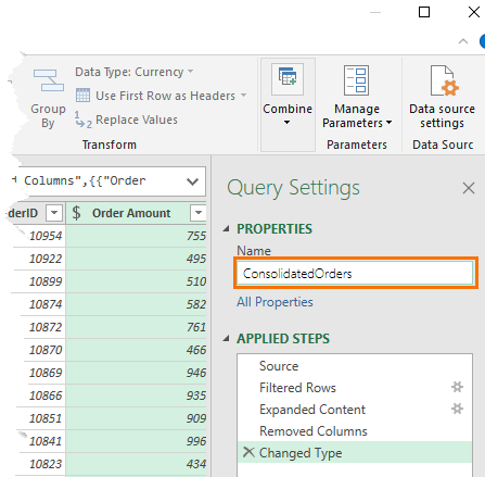
Step 8:
Now we’re ready to load the data into Excel or Power Pivot. On the Power Query Editor Home tab > Close & Load > Close & Load To…: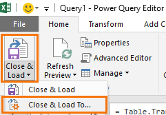
Step 9:
Choose the destination for your data: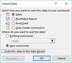
Note: Excel 2010 and 2013 will not have PivotTable Report or PivotChart, as listed above. Excel 2010 will not have the ‘Add his data to the Data Model’ option.
I chose to load my data into a Table in a new worksheet, as you can see below:
It’s important to note that Power Query does not alter the original tables. It merely takes a copy of the data and creates a new table for you to work with. If data in the original tables gets updated, you can simply refresh the query (Data tab > Refresh all) and it will update the consolidated table.
You can also get the data from other Excel files and create a new file for the consolidated data. This helps keep your file size manageable if you’re working with a lot of data.
Learn More Power Query
Everyone should learn Power Query. It really is a game changer for automating tasks and making light work of laborious jobs.
So, if you’d like to learn Power Query take a moment to check out my course:
- It’s available for accountants and other professionals who require CPE credits through Excel University with 12 CPE credits.
- Or if you don’t need CPE credits you can get it for less here on my site here.


Hi! How can I split a worksheet into different files?
thanks!
Hi Mayra,
Here is an article that provides a solution for that scenario, you can download the sample file to test it.
I want to stack only one sheet from multiple workbooks by power query. The sheets are identical in all the workbooks
Check out this tutorial on importing multiple files containing multiple sheets with Power Query.
Hi Mynda, first of all many thanks for sharing this amazing knowledge with us. But please I have an issue, where every time I try to refresh the query whether using Refresh All or Refresh selected data only, I get all inserted data from all tables inserted again underneath the original ones, and when I try to remove the duplication it keeps the updated row, could you please advise how to avoid this issue.
Hi Peter, you need to remove the output query from being picked up in the query itself by filtering it out after the ‘source’ step.
Mynda
Thanks for your reply but it seems that I don’t know how to do so. I would appreciate if you can share some snapshots to show me how to do so.
Hi Peter, please post your question and sample Excel file on our forum where we can help you further.
Hi! The first time I tried this query, it worked like a charm. The second time though, I hit a roadblock. II have 30 tabs and I see them all listed in the query, but when I try to expand to see all the info from all the tabs, only one tab shows up. Any idea what I could be doing wrong? Thanks a lot!
Hi Ann, not without seeing the file. Can you please post your question on our Excel forum where you can share it, or at least some screenshots and the M code.
Mynda
Thank you, is there a way to convert multiple worksheets data range into tables? i have 200 plus tabs and converting them one by one will take a lot of manual effort and it’s a repeated process.
Any suggestion would be greatly appreciated.
thank you
Hi Afia,
If you use Get Data > From Folder, you don’t need the data formatted in a Table. Simply navigate to the folder path > Transform. In the query editor remove all except the Content column. Then add a column with the following formula:
=Excel.Workbook([Content])
You can then expand that new column to see the sheets. Apply a filter to keep only the sheets you want. Then remove all columns except the Content column and maybe the sheet names column. Then expand the Content column to consolidate the data.
Mynda
This was just what I needed! I got a mess with each month on different pages and each column ever so slightly different every month or two and this made it niiiiice and easy!
Glad we could help, Maria 🙂
Very happy to have discovered this excellent tip!
My Excel solution queries 3 data sources (each returning 1,000’s of JSON records) and merges their results into a 4th query.
Before discovering this tip, each time I refreshed my 4th “Merge” query, it triggered time-consuming re-refreshes of the 3 JSON queries.
After implementing the solution described in this tip, when I refresh my 4th “Merge” query it does not cause the 3 JSON queries to refresh.
Thank you!
Glad it was helpful, Brian 🙂
=Excel.CurrentWorkbook() does not show a list of worksheets in the workbook I am trying to use this feature on. Can you explain why?
The workbook needs to contain an Excel Table, Named Range or Filtered List for Power Query to be able to find the data in your file.
Excel.CurrentWorkbook() does not show a list of worksheets in a workbook, why is that? sometimes we need complex calculations to be done in worksheets for a specific problem and you may not want to convert data into an Excel table or named range?
Try Excel.Workbook(CurrentWorkbookPath), this will give you the content.
Good morning Mynda,
Thank you for very helpful videos to get my data in the correct form and then to use Power BI. I would like to ask help with one specific graph tool; “Line and Stack Column Chart”. I have four data points under my Sample ID field. I would like to use 3 of the points as the stack column chart and the fourth entry of the Sample ID for the Line Chart. I am not sure if this makes sense. In essence If I have four Reps, I would like the show the sales of 3 reps as a stacked column chart and the four rep as the line chart. Could you please assist?
Hi Kobus,
That’s an interesting idea. It’s not something you can do with native charts. You’d have to plot the line as a separate series with a value for each of the 3 sales reps that are displayed as columns in the chart (not stacked). It’s tricky to describe, but if you want to post your question on our Excel forum with a sample file we can show you.
Mynda
Hi Mynda,
Thank you for sharing this. Will this process work if the total rows of the combined table exceed the 1,048,576 Excel row limitation for 1 sheet?
Kind regards,
Ed
Hi Ed,
Yes, you can consolidate sheets where the total data exceeds the Excel sheet limit, but you’ll have to ‘Close & Load’ it to the Data Model/Power Pivot as this can store millions of rows. From there you can create PivotTables to summarise and analyse the data.
Mynda
Is it possible to do this without having named ranges or tables defined? If I created a new workbook, I could create a connection to this workbook and could then transform the data with Power Query. No named ranges or tables would be needed. I’m curious what it would take to do this type of import from inside the main workbook.
Hi Ben,
You will always be able to choose to import data from named ranges, or tables, or sheets, even if the sheet contains exactly the same data as the defined table. When you select a workbook to import data from, you will have a column that will display the type of data found in that workbook: names, tables, sheets. (the column name is ‘Kind’)
I did some more searching and found a post on Excel UserVoice that fits what I was trying to say. I would be nice if Excel.CurrentWorkbook would return the same items as Excel.Workbook. If it did, we could refer to the contents of a sheet without having a named range or table on it. I have also read that there are some workarounds, but they have limitations like having to save the file before you can refresh the Power Query steps.
https://excel.uservoice.com/forums/304921-excel-for-windows-desktop-application/suggestions/15673497-harmonize-excel-currentworkbook-with-excel-workboo
After seeing it on UserVoice, I see that I’m not the only person who wants this feature. Please go there and vote for it too!
Hi
thanks for this. After combining the data, I added a new column to one of the tabs, i tried refreshing but this wasn’t picked up in the combined data. Is there something else i need to do for the new column to be added to the combined data?
thanks for your help.
Hi Amiee,
Depends on how your query is built. Check the query text, see if column names are hard typed in text, if so, you will need to make the column names list dynamic.
Use our forum to upload a sample query, to see what can be done.
One of the consolidation rules are that “The table structure (column names) on each sheet you want to consolidate are the same.”
But what if they’re not the same? For example, let’s say I want to add data from a five-column table to a ten-column table. The five-column table’s headers are the same as the larger table’s, but it’s missing five columns for which there is no data. In the columns for which data is missing, I want the new, appended table to show blanks or nulls. Is this possible? The only workaround I can think of is to add five columns to the smaller table so that the headings are the same in both tables, then append as normal.
Hi Paul,
You can still append, it will add the columns with different names instead of appending them.
Mynda
Thanks Mynda.
I am going to have fun with this new add-in. I am trying to reckon how it will help me consolidate data from different (10) account reports. However, I had a hitch in that when I work with pivot tables, which I do a lot, I cannot view the design and format tabs for pivot tables. Is there a reason why? Is there any way to restore this situation without disabling or uninstalling Power query?
Many thanks.
Hi Anne,
Those context tabs in ribbon are visible only when you select any cell within a pivot table range. If you select any cell outside the pivot range, those tool tabs will not be displayed.
If you’re sure that a cell from pivot range is selected, and those tabs are not visible, make sure it’s really a pivot and not a range copy pasted from a pivot that only has the look of a pivot table.
Regards,Catalin
Thanks for showing how to use the Excel.CurrentWorkbook() function.
Glad you liked it, Joan. Have fun with Power Query. It is a life changer 🙂
This is wonderful and informative. Thank you for the chronological way of explaining the power querry.
Thanks, Mohamed! Great to know you found it helpful.