There’s no built-in way we can force Excel Slicers to single select, but we can use some crafty tricks to prompt users to only select one item, and even hide the data if they try to select multiple items!
Watch the Video

Download Workbook
Enter your email address below to download the sample workbook.
Force Excel Slicers to Single Select – Option 1 for Regular Charts
Step 1 – Add a dummy PivotTable containing the Slicer field in the row labels
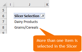
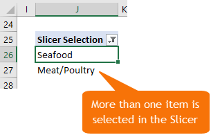
In my example it’s the Category field. If only one item is selected, cell J8 will be empty. You can see in the image below that two items have been selected in the Slicer:
Note: ensure the Slicer is connected to both the PivotTable feeding your chart data and the dummy PivotTable by right-clicking the Slicer > Report Connections. In the dialog box choose all PivotTables that the Slicer should be filtering.
Step 2 – Test if cell J8 is blank
You can use an IF formula to test if the second row in the PivotTable is empty (shown below in cell L7). If it is, return the text you want displayed in the chart title. If it’s not blank, have it return a message for the user:
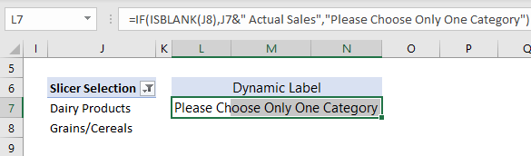
Note: you can use J8="' in place of ISBLANK(J8) if you prefer.
Step 3 – Link Chart Title to IF Formula Result
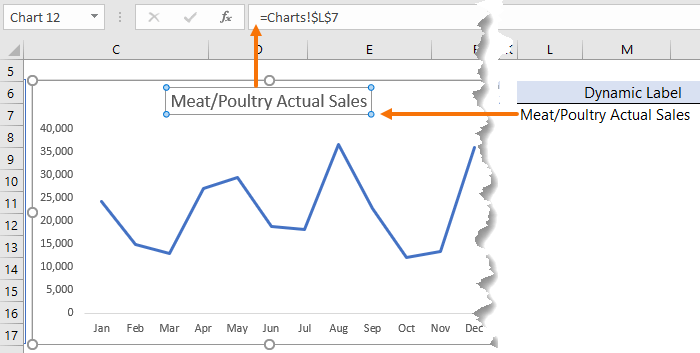
Select the chart title, then in the formula bar reference cell L7, containing the IF formula result:
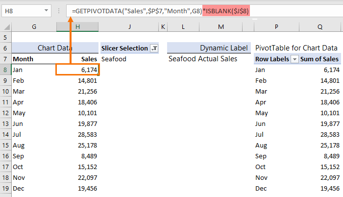
Step 4 – Multiply chart values by ISBLANK
You can use the same ISBLANK test to hide the values for the chart if cell J8 is not blank. Simply multiply the GETPIVOTDATA formula with ISBLANK, which returns a TRUE if it’s blank and FALSE if not. When you multiply Boolean TRUE/FALSE values, TRUE becomes 1 and FALSE becomes 0:
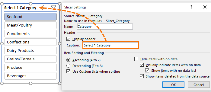
Step 5 – Use Slicer header for instructions
Right-click the Slicer > Slicer Options > edit the ‘Display Header’ instructing your users to only select 1 item:
Force Excel Slicers to Single Select – Option 2 for Pivot Charts
With PivotTables we can’t hide the data in the chart, so we need to get more in your face with the chart title message:
The first two steps are almost the same. Note that this example is further down the worksheet, starting on row 25.
Step 1 – Add a dummy PivotTable containing the Slicer field in the row labels
In my example it’s the Category field. If only one item is selected, cell J27 will be empty. You can see in the image below that two items have been selected in the Slicer:
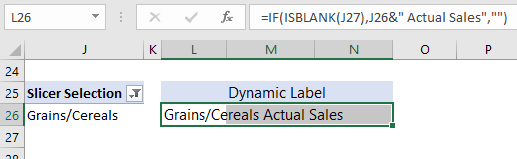
Step 2 – Test if cell J27 is blank
You can use an IF formula to test if the second row in the PivotTable is empty (shown below in cell L26). If it is, return the text you want displayed in the chart title. If it’s not blank, hide the label with blank as denoted by two double quotes:
Note: ensure the Slicer is connected to both the PivotTable feeding your chart data and the dummy PivotTable by right-clicking the Slicer > Report Connections. In the dialog box choose all PivotTables that the Slicer should be filtering.
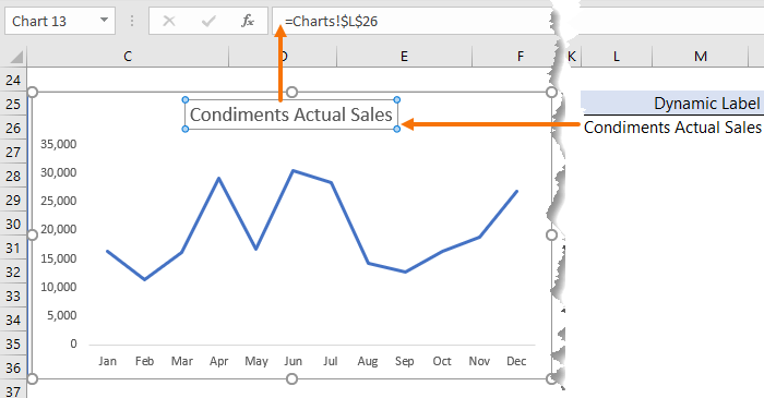
Step 3 – Link Chart Title to IF Formula Result
Select the chart title, then in the formula bar reference cell L26, containing the IF formula result:
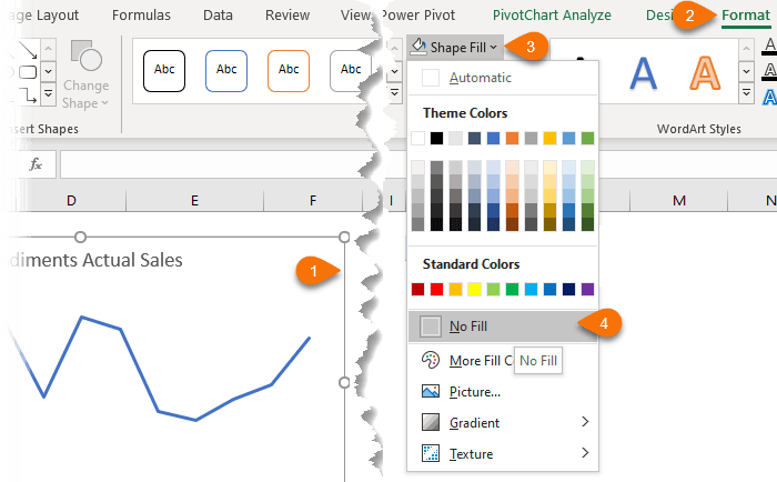
Step 4 – Remove chart fill
Select the outer edge of the chart > Format > Shape Fill > No Fill:
Step 5 – Insert IF formula behind chart
In an empty cell behind the chart, insert an IF formula that checks if the second row of the PivotTable is blank. If it is blank, the formula returns nothing, otherwise it returns a message for the user in font formatted red and bold:
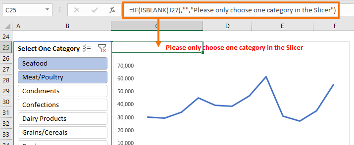
When only one item is selected in the Slicer this message doesn’t display and the chart title is visible. When two or more items are selected, the chart title returns a blank and the message behind the chart is visible.
Step 6 – Use Slicer header for instructions
Right-click the Slicer > Slicer Options > edit the ‘Display Header’ instructing your users to only select 1 item:
More on Slicers
 |
Get started with Excel Slicers - Slicers, introduced in Excel 2010, are an interactive control that enables you to filter data in PivotTables, PivotCharts, Excel Tables and CUBE functions. |
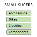 |
Excel Slicer Formatting - with these hidden settings you can make Slicers very small, allowing you to fit them into crowded dashboards. |
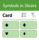 |
Symbols in Excel Slicers - Did you know you can display symbols in Excel Slicers? That’s right, Slicers aren’t just limited to listing boring old items from your PivotTables or Tables. |
 |
Reference Slicer selection in formulas - Slicers are a great tool for incorporating interactivity into your reports but we don’t always want to analyse our data with PivotTables and PivotCharts. Nor is our data always in the perfect format for PivotTables. |


Hello Mam,
First of all i thank you for your videos. I really learn a lot from your videos.
Here I need your favor, i am facing the following problem.
how can Force Excel Slicers to Single Select for pivot charts having primary and secondary axis? Because if a chart is having primary and secondary axis then when selecting multiple items from the slicer then the chart view got changed and also when we feed new data to the source then it automatically selects all items in the slicer and the chart got changed and i need to do the visualization again.
Thanks in advanced.
You can’t force Slicers to single select for Pivot Charts, so you’re best to build a regular chart from the PivotTable.
hi!
Do you know how to do the opposite, ie have the multislicer automatically selected by default? I look and look on the web but I found nothing.
My file is for users unfamiliar with slicers. They will disregard the tool if they cannot select more than one item!
Thanks for everything I learnt through your videos. your work is outstanding.
Hi Celine,
Slicers are multi-select by default. You just have to know how to do it! You can left click and drag to select multiple items or hold CTRL and left click to select non-contiguous items. Alternatively, in later versions of Excel you can turn on the ‘multi-select’ toggle in the header of the slicer beside the clear filters button to allow users to multi-select with a single left click.
Mynda
One alternative: (requires VBA)
1) Build your slicer(s) as usual. For the slicer that you want to make single-select, do the following:
2) Using Developer / Design Mode / Insert / ActiveX : Add a Radio button to your sheet for each option you want the user to choose. (Hint: Use the Properties / caption to customize the label.)
3) Double click the radio button to launch the “optionbutton1_click” macro in the VBA editor.
4) Insert a macro like the one here, replacing “slicer_name” with the name of your single-serve slicer, and “option#label” with the actual label names that are on your slicer:
ActiveWorkbook.SlicerCaches(“slicer_name”).ClearManualFilter
With ActiveWorkbook.SlicerCaches(“slicer_name”)
‘ Set only 1 option TRUE (coordinate with your radio button label); set all others FALSE:
.SlicerItems(“option1label”).Selected = True
.SlicerItems(“option2label”).Selected = False
.SlicerItems(“option3label”).Selected = False
(repeat as needed, setting all others to FALSE)
End With
5) Repeat step 3+4 for each radio button, setting the correct TRUE/FALSE for the appropriate option each time. (i.e. your 2nd macro would set the 1st option FALSE, and the 2nd option TRUE, etc)
6) HIDE your Slicer so the user can’t see it to make their own selections. Use ALT+F10 to open the “Selection” window, and click the “eyeball” icon next to your slicer name to hide it.
The radio buttons can now be placed, organized, customized, and formatted as needed to fit your aesthetic.
Thank you Glenn for sharing, looks good
Cheers,
Catalin
Hi Glenn,
Thank you for your sharing.But I use OLAP data source (the data model), and I keep getting Error “1004 – Application-defined or object-defined error” when I try to use your code.
Could you help here? thx
Rita
I suggest recording a macro to get the proper syntax that can be used in that code, everything in this page refers to normal pivot tables, not power pivots.
Thanks for the tips.
.
Any reason why you did not mention the “multi-select” button and context menu option?
.
Turn Slicer into a “radio button” selection- “Multi-Select” Button / Option
In the upper right corner of the slicer there are 2 buttons. Click on the one with the check marks, “Multi-Select button, to toggle the single select, “radio button” / multi selection option.
You can also toggle this option by right clicking on the Slicer to display the context menu. Click on the “Multi-select” option in the context menu. Unfortunately, at this time that entry is NOT highlighted when it is selected. You have to look at the slicer for the subtle shading to indicate if it is selected not.
.
I tried to submit a Feedback, but it just clocked, did not save …
Hi Ron,
Great question. The multi-select button is not what it appears…this button is for allowing users on touch screen devices to multi-select items by clicking on them one at a time. By default, to select multiple items you click on the first item, then to select another item you must hold down Shift, or CTRL, or left click and drag. With touch screens you simply toggle the multi-select button on to allow you to select multiple items by touching one item at a time. Hope that clarifies things.
Mynda