Symbols in Excel Slicers

Did you know you can display symbols in Excel Slicers? That’s right, Slicers aren’t just limited to listing boring old items from your PivotTables or Tables.

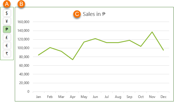
In the animated image below I’ve got a Slicer that displays currency symbols. As you click on a currency symbol in the Slicer, the chart converts to the selected currency.

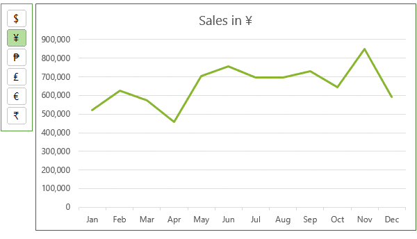
Of course, this isn’t limited to use with charts and in fact this isn’t even a PivotChart. Let your imagination run wild…why not use this technique to convert a whole dashboard into different currencies.

Watch the Video

Download the Workbook

Interactive Chart with Symbols in Excel Slicers

There are just 4 components to this example so let’s step through them and then we’ll look at some other examples of symbols in Excel Slicers.

Step 1: Currency Table

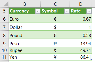
The table above, called tbl_currency, contains the list of currencies and their exchange rate.

The Symbols are found on the Insert tab > Symbol:

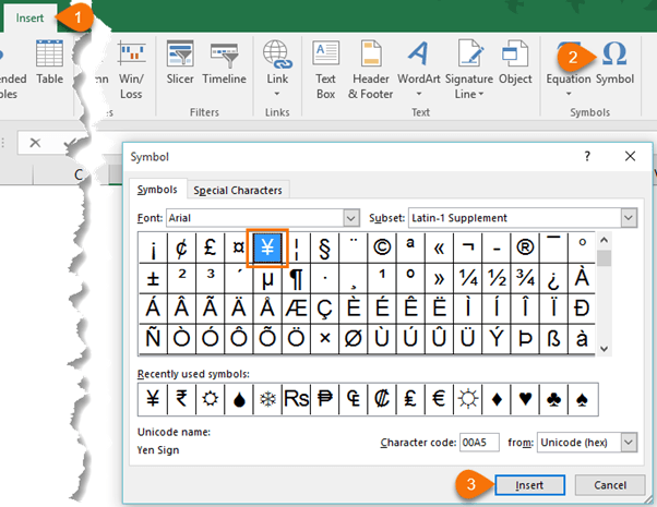
Note: Symbols using Wingding fonts require special treatment. More on that later.

Step 2: Insert a PivotTable & Slicer

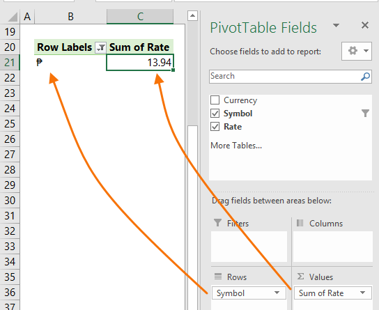
The source data for the PivotTable in cells B20:C21 is tbl_currency.

A Slicer for the PivotTable Symbol field allows the user to specify which currency is displayed in the chart and filters the PivotTable to only display one currency. How to insert and use Slicers.

Step 3: Sales Table for the Chart

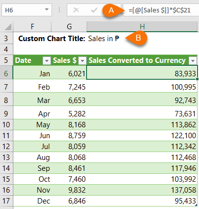
The table above (called tbl_chartData) contains the sales by month. Columns F and H feed the chart.

a. Column H converts the sales into the currency based on the symbol selected in the Slicer, the rate for which is in cell C21 of the PivotTable. Notice that the formula uses Structured References ( [@Sales $]] ) because this is an Excel Table. More on Tables and Structured References here.

b. Cell H3 (above the table) contains a custom label for the chart title that picks up the currency symbol selected in the Slicer. How to insert custom chart labels.

Note: If multiple currencies were selected in the Slicer it would convert it to the first currency selected. Any other selected currencies would be ignored because the formula in column H is only interested in the rate in cell C21.

Step 4: Insert Chart and Format Slicer

a. Position the Slicer beside the chart. Remove the Slicer header (right-click Slicer > Slicer Settings > uncheck ‘Display Header’).

Tip: Slicers can be on a different worksheet to the PivotTable.

b. Insert the chart; select column F and H of the table (hold CTRL to select non-contiguous cell ranges) > Insert tab > Charts - select a line (or column) chart.

c. Link the Chart Title to the custom label in cell H3. Tutorial on Custom Chart Labels.

Summary

There are just 5 skills required to create this interactive chart:

1. Excel Tables and formulas using Structured References (this is recommended, but optional. A regular table would work too).
2. Excel PivotTables
3. Slicers
4. Inserting Charts (nothing complicated, just use the charts on the Insert tab)
5. Custom Chart Labels

So, you see that even with some quite basic Excel skills you can create something clever. In my Excel Dashboard course I aim to equip you with lots of skills that you can combine to create powerful reporting solutions to wow your users.

Other Symbols in Excel Slicers

There are tons of different symbols available in the Insert Symbol dialog box, but you must watch out for symbols that require a special font. This is because Slicers have a default font and if you want something special then you have to create a custom Slicer Style (more on that later).

Here are some examples:

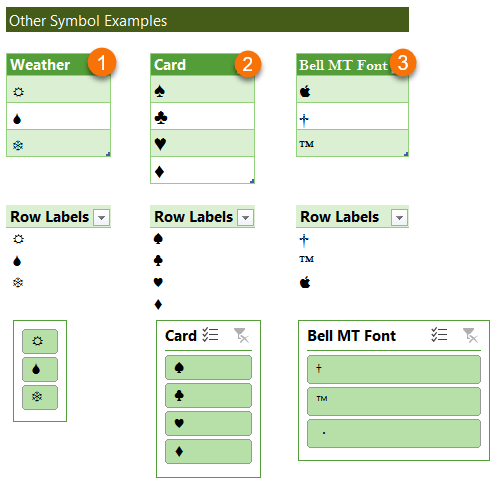
1. The weather symbols use Wingdings. We need to set up a custom Slicer Style for these to render properly in the Slicer. More on that in a moment.
2. The Cards are fine, they just use Arial font. Note: if you don't see these symbols in the Symbols dialog box, you can enter them using the Windows Character Map program.
3. The last example uses Bell MT. You can see that the apple symbol doesn’t render in the Slicer but the other two do. Again, this Slicer will require a custom Slicer Style if you want to use these symbols.

Caution: If you require a custom Slicer Style then you can only choose symbols from the same font family, because you can only set one font for the Slicer buttons.

Creating Custom Slicer Styles

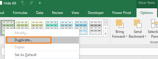
Creating a Custom Slicer Style is easy and it travels with the Excel file:

1. With a Slicer selected go to the SlicerTools: Options tab > right-click an existing Slicer Style that you like the colour scheme of > Duplicate:

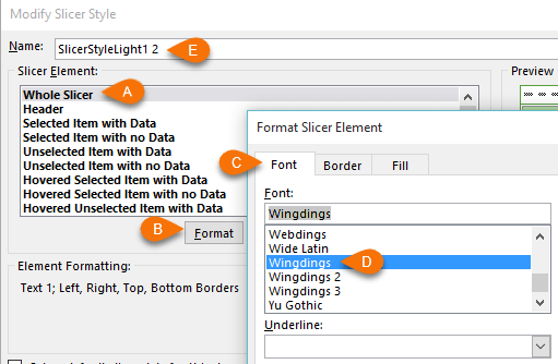
2. In the Modify Slicer Style dialog box (image below), we’ll set the font for the Slicer



a. Select the ‘Whole Slicer’ element

b. Click the ‘Format’ button.

c. Go to the Font tab

d. Choose the font to match your symbols

e. Give your Slicer Style a name if you want.



Bonus tip: if you want your Slicer header to display in a regular font, like Arial, choose the ‘Header’ Element and change the font back to something readable.

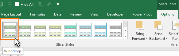
3. Apply your custom Slicer Style to the Slicer: Select the Slicer > SlicerTools: Options tab > in the Slicer Styles gallery click on your custom style. Tip: It should be the first one in the list:

Thanks

I stumbled upon this post by Rob Collie on using Wingdings in Slicers for Power Pivot, which was the inspiration for this post.