Combine Excel Worksheets with Power Query

A recurring task in my previous life as an accountant was to analyse actual vs budget figures.

However the figures were often in different worksheets, different workbooks or even different systems. And the task of consolidating all the data into one table that was ready to analyse with PivotTables was not straight forward.

Not anymore. It’s a doddle now that Excel has Power Query*. So let’s take a look at how to combine Excel worksheets with Power Query.

Download the Workbook

Watch the Video

Change settings to HD for best viewing.

Combine Excel Worksheets with Power Query - Written Tutorial

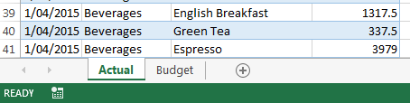
For this example the data is nicely formatted in Excel Tables in one Excel workbook, with separate sheets for the Actual and Budget figures:

Note: your data might not be so well behaved, but don’t worry. Power Query can get data from almost anywhere, including multiple files, folders, systems etc. More on that later.

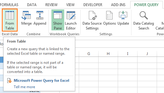
Load to Power Query

Next we need to load the two Tables into Power Query. We can use the ‘From Table’ tool on the Power Query tab of the Ribbon to load one Table at a time:

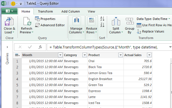
After clicking the ‘From Table’ button the Query Editor opens and you can see a preview of your data:

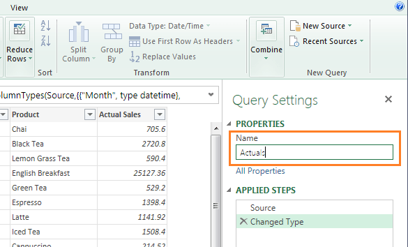
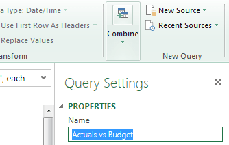
In the Query Settings change the Name of your Query to something meaningful. I’ll call mine ‘Actuals’:

Click the ‘Close & Load’ down arrow and select ‘Close & Load To’:

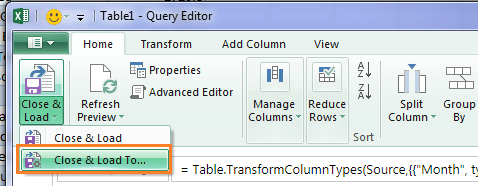
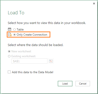
And in the ‘Load To’ dialog box select ‘Only Create Connection’:

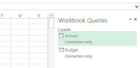
Repeat for the Budget sheet so you now have 2 queries in your workbook. You can see mine in the Query pane on the right-hand side of the screenshot below:

Append the Queries

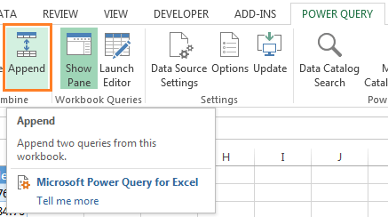
Next we need to append the queries together.

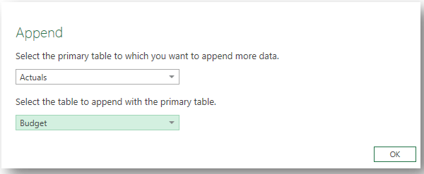
On the Power Query tab select ‘Append’:

In the Append dialog box select the two query tables and click OK:

Note: You could Merge the queries (as opposed to Appending). However if you have budget figures without corresponding actuals and vice versa then you must use append, otherwise you’ll lose some data.

The Query Editor will open and you can see a preview of the appended queries. Notice how the Budget column contains a load of null values? This is because the Actuals are at the top, but if I were to scroll down I’d see the budget values.

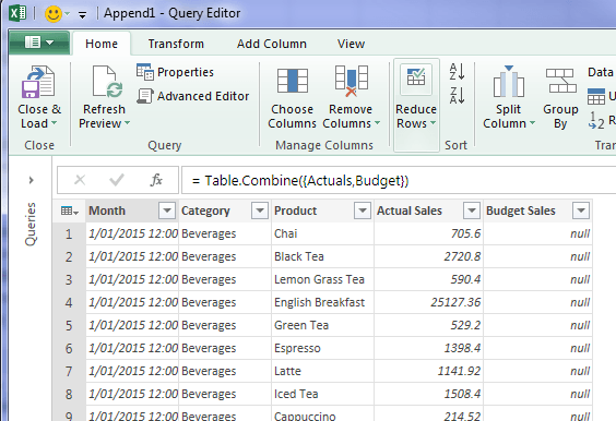
So far this isn’t a lot better than copying and pasting the two tables under one another. Ideally we’d like the corresponding budget figures to be on the same row as the actuals.

Group Rows

We can use the ‘Group By’ tool to do that. On the Transform tab of the ribbon you’ll find Group By button:

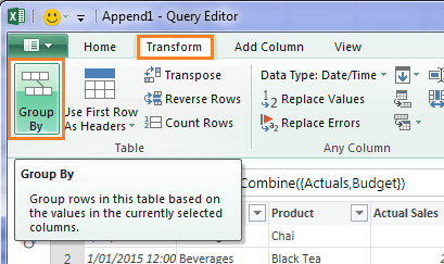
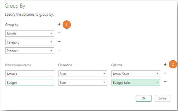
Clicking it opens the Group By dialog box (image below) where you can:

1. Add the columns you want to group together (tip: select the columns before clicking ‘Group By’ to save a step).
2. Tell Power Query how you want the other columns summarised.

Use the +/- buttons to add and remove columns.

Now you can see a preview of your grouped data:

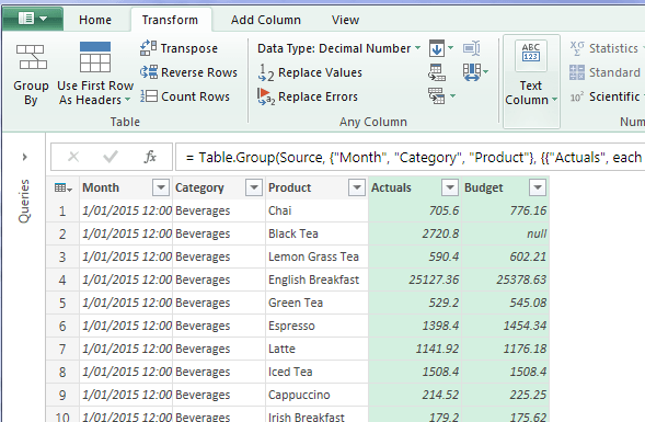
Notice how the second row has a null budget value? This is because we have an actual for Black Tea in January, but no budget.

Rename Query

I’ll give the query a more meaningful name by typing over the default in the ‘Name’ field in the Query Settings pane of the Query Editor:

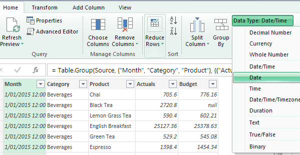
Set Data Types

Now we can set the data types before we put the data into an Excel Table or Power Pivot. This is particularly important if you’re putting the data into Power Pivot, as the data types will flow through.

On the Home tab you’ll find the ‘Data Type’ menu. Simply select each column in turn and set the type from the list:

In the Query Settings pane under ‘Applied Steps’ we can see all the steps we’ve taken so far to:

1. Append the queries
2. Group the rows and
3. Set the data types

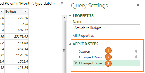
These steps are saved with the query. And this means if the data in our original tables changes, or we get new data, like Actual figures for the previous month, then we can simply refresh the query and Power Query will get the data. It runs it through all the steps in the query without us having to do a thing!

Close & Load

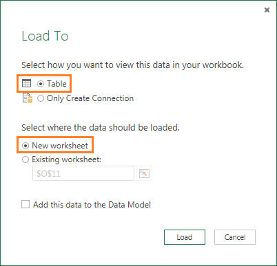
We’re ready to Close & Load our data to an Excel Table, and or Power Pivot. I’m going to put it straight into a Table in the current file on a new worksheet so at the ‘Load To’ dialog box I’ve selected ‘Table’ and ‘New Worksheet’:

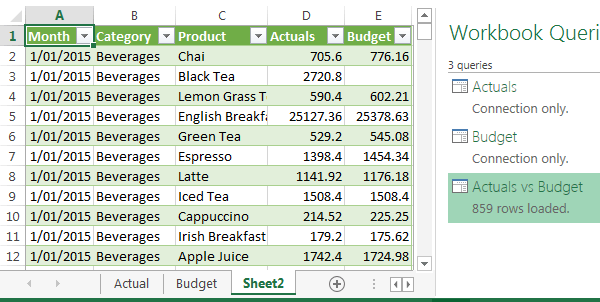
You can see I’ve got a new sheet (Sheet2) with my appended data, and in the Queries Pane I have a 3^rd query (Actuals vs Budget) in the file:

Now you can go ahead and analyse the data in PivotTables etc.

Athough there were a lot of steps in this tutorial, I'll think you'll agree it's pretty easy to combine Excel Worksheets with Power Query.

Refreshing the Queries

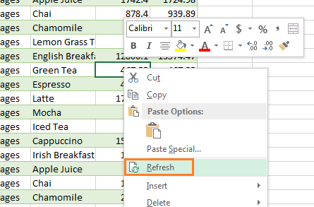
If any data changes in our Actual or Budget tables we can press CTRL+ALT+F5 to refresh everything, or right-click a cell in the Actuals vs Budget query table and select ‘Refresh’:

Data Sources

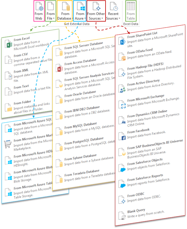
In this example the data was conveniently housed in one Excel workbook and nicely formatted in Excel Tables. If your data isn’t so well behaved, fear not, Power Query can get data from almost anywhere, including multiple different sources:

Learn Power Query

I can’t think of a job involving Excel where you wouldn’t benefit from Power Query. It is the most exciting Excel tool since PivotTables, not just because it’s so powerful, but also because it’s useful for everyone.

In my Power Query course I’ll get you up to speed fast, so please take a moment to click here and check it out and see another video of Power Query in action.