• Skip to main content
  • Skip to header right navigation
  • Skip to site footer

My Online Training Hub

Learn Dashboards, Excel, Power BI, Power Query, Power Pivot

  • Courses
  • Pricing
    • Free Courses
    • Power BI Course
    • Excel Power Query Course
    • Power Pivot and DAX Course
    • Excel Dashboard Course
    • Excel PivotTable Course – Quick Start
    • Advanced Excel Formulas Course
    • Excel Expert Advanced Excel Training
    • Excel Tables Course
    • Excel, Word, Outlook
    • Financial Modelling Course
    • Excel PivotTable Course
    • Excel for Customer Service Professionals
    • Excel for Operations Management Course
    • Excel for Decision Making Under Uncertainty Course
    • Excel for Finance Course
    • Excel Analysis ToolPak Course
    • Multi-User Pricing
  • Resources
    • Free Downloads
    • Excel Functions Explained
    • Excel Formulas
    • Excel Add-ins
    • IF Function
      • Excel IF Statement Explained
      • Excel IF AND OR Functions
      • IF Formula Builder
    • Time & Dates in Excel
      • Excel Date & Time
      • Calculating Time in Excel
      • Excel Time Calculation Tricks
      • Excel Date and Time Formatting
    • Excel Keyboard Shortcuts
    • Excel Custom Number Format Guide
    • Pivot Tables Guide
    • VLOOKUP Guide
    • ALT Codes
    • Excel VBA & Macros
    • Excel User Forms
    • VBA String Functions
  • Members
    • Login
  • Blog
  • Excel Webinars
  • Excel Forum
    • Register as Forum Member

Calculating MEDIAN in PivotTables

You are here: Home / Excel PivotTables / Calculating MEDIAN in PivotTables
PivotTable Median
October 27, 2015 by Mynda Treacy

Unfortunately there’s no built in way to calculate the median in a PivotTable. The approach is different depending on whether you’re using a regular PivotTable or a Power Pivot PivotTable. We’ll look at both options in this tutorial.

The Data

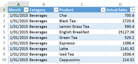
The data we’ll be using in this example is in an Excel Table called Table1:

data for calculating median in PivotTables

Download the Workbook

Enter your email address below to download the sample workbook.

By submitting your email address you agree that we can email you our Excel newsletter.
Please enter a valid email address.

  • Download the Excel 2013/2016 Workbook.
  • Download the Excel 2010 Workbook.
Note: These are .xlsx files, please ensure your browser doesn't change the file extension on download.

Calculating Median in PivotTables

We’ll look at calculating the Median in a regular PivotTable first. It’s not actually ‘in’ the PivotTable, but rather in a spare column to the right of your PivotTable.

In the image below you can see my PivotTable is in columns B and C, and I’ve put my median formula in column D. I’ve formatted the header in cell D7 with blue fill to make it appear part of the PivotTable, but you if you look in the formula bar you'll see the formula:
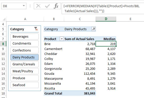
pivottable median formula

The formula is:

=IFERROR(MEDIAN(IF(Table1[Product]=Pivots!B8,Table1[Actual Sales])),"")

It’s an array formula so it’s entered with CTRL+SHIFT+ENTER, which automatically inserts the curly braces you can see surrounding the formula in the formula bar above.

Let’s look at each component of the formula starting with IF:

The IF formula returns an array of values from the Table1 Actual Sales column IF the Product column contains the value in B8 (Brie), of the PivotTable.

In English it reads: if the product is Brie, then return the value from the Actual Sales column.

These values are then passed to MEDIAN which simply returns the median value.

In the event that the formula returns and error, IFERROR will override it and return nothing, as denoted by the "" at the end of the formula:

=IFERROR(MEDIAN(IF(Table1[Product]=Pivots!B8,Table1[Actual Sales])),"")

IFERROR allows me to copy the formula down to row 20, to allow for growth or contraction in the PivotTable that may occur as a result of changes in the Slicer selection, and prevents an error showing in the event of missing data.

Calculating Median in Power Pivot

In Power Pivot we can call on the DAX formula language to write our own median formula that we can use inside a PivotTable (see column I below):

DAX median formula

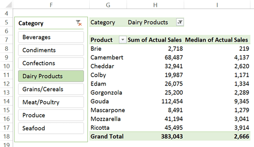
These DAX calculations are known as Measures (in Excel 2013 they are called Calculated Fields). The advantage of using Measures is that we can use the median calculation in the values area just as we would any other item in the field list.

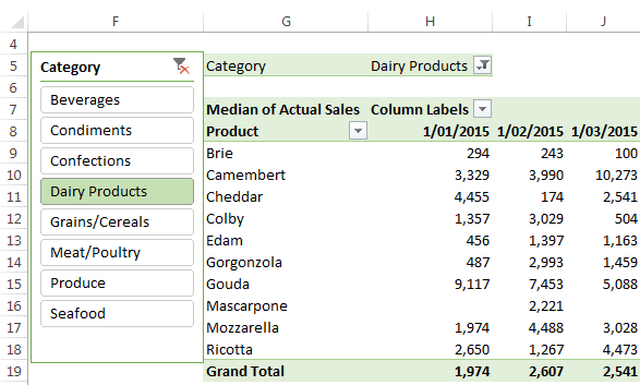
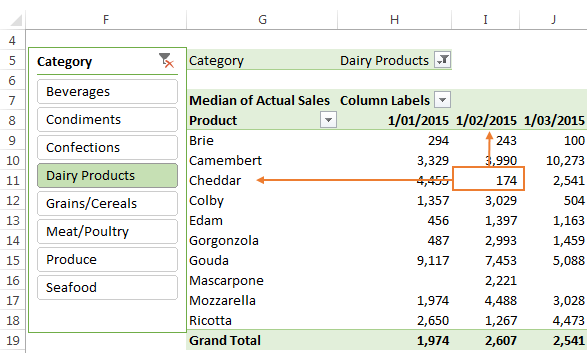
For example, I can easily add the Month field to the columns area to find the median for each product by month:

power pivot DAX median formula

This flexibility is not available as easily with the formula approach for regular PivotTables that I showed you above. However, with flexibility comes a bit more complexity. Let’s look at how to write the Median formula in Power Pivot's DAX formula language and create the new measure/calculated field.

Inserting a DAX Measure

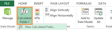
There are a few places you can insert your measure; in Excel 2013 we’ll use the ‘New Calculated Field’ menu on the Power Pivot tab of the ribbon:

insert calculated field power pivot excel 2013

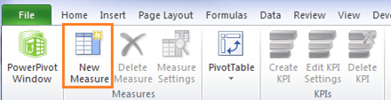
In Excel 2010 it’s called ‘New Measure’:

insert new measure power pivot excel 2010

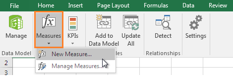
And in Excel 2016 it’s also ‘New Measure’:

insert new measure power pivot excel 2016

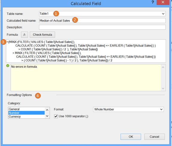
This opens the Calculated Field (measure) dialog box where we:

  1. Assign the measure to a table, which is usually the table containing your transactional data. I only have one table in my model, called Table1.
  2. Give your measure a name
  3. Enter your formula
  4. Set your formatting and data type

insert dax formula

DAX Median Formula

Ok, let’s address the formula elephant in the room! I know that formula may look a little large, and maybe even daunting.

Fear not. DAX is similar to the Excel formula language, but it has some different functions, and unlike Excel functions, DAX is case sensitive.

Here is the DAX MEDIAN formula (line breaks have been added to help readability):

=(
MINX(
FILTER( 
VALUES( Table1[Actual Sales] ),
CALCULATE(
COUNT( Table1[Actual Sales] ), Table1[ActualSales] 
<= 
EARLIER( Table1[Actual Sales] ) )
> 
COUNT( Table1[Actual Sales] ) / 2 ), Table1[Actual Sales])
+ 
MINX( FILTER ( VALUES ( Table1[Actual Sales] ),
CALCULATE(
COUNT( Table1[Actual Sales] ), Table1[Actual Sales] 
<= 
EARLIER( Table1[Actual Sales] ))
>(
COUNT( Table1[Actual Sales] ) - 1 ) / 2 ), Table1[Actual Sales])) / 2

I know it looks scary, but there should be some familiar features, like:

  1. It looks similar to an Excel formula; after all, it starts with an equals sign 😉
  2. There are parentheses surrounding each function and commas separating arguments
  3. It uses the same type of operators, like >, =,-, /
  4. It uses Structured References just like an Excel Table e.g. Table1[Actual Sales] references the Actual Sales column of Table1.
  5. It even has the COUNT function, just like in Excel!
  6. It only references one column; the Actual Sales column, so it’s easy to copy and paste it into your own model and simply edit the Table_Name[Column_Name] components in red to suit.

See, easy! 😉

Notes:

  • This formula may be slow on very large data sets.
  • In Excel 2016 there is a new MEDIANX DAX function, which means we can replace the elephant sized formula above with this much simpler and more efficient formula.
    =MEDIANX( Table1, Table1[Actual Sales])

Measures Obey Context

You might be wondering how the DAX median formula calculates a different value for each cell in the PivotTable when it only references one column in the formula (the Actual Sales column).

This is because most DAX functions recognise the context of the column and row labels for each cell and automatically apply those filters to the formula. For example; in cell I8 of the PivotTable below the DAX median function is only calculating the median for Brie:

dax formula context

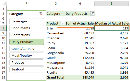
Another way to think of context is similar to an IF function e.g. the median in cell I8 above is much like the MEDIAN(IF… formula I used in the very first PivotTable, except with DAX I didn’t have to write the IF part. The measure did that all by itself based on each value cell’s location in the PivotTable.

Similarly, in cell I11 of the PivotTable below the DAX median function is only calculating the median for Actual Sales IF the Product is Cheddar and the date is 1/02/2015 (d/mm/yyyy):

dax formula filters with context

This flexibility in DAX measures is one of the reasons they’re so powerful. We can build them once and use them again and again.

And since they only calculate on demand, they don’t bog down our file with memory intensive calculations.

Get and Learn Power Pivot

Power Pivot is available as a free add-in in Excel 2010, or Excel 2013 Office Professional Plus, Office 365 Professional Plus, or in the standalone edition of Excel 2013. Note: it is built into Excel 2016 Professional Plus and the standalone Excel 2016 so you don't need to install an add-in.

Power Pivot is not available in Excel for Mac.

If you’d like to learn Power Pivot and DAX formulas, please take a moment to check out my Power Pivot course.

Thanks

Thanks to Marco Russo and Alberto Ferrari at DAXpatterns.com for a wonderful resource on DAX measures, which is where I got the DAX Median formula.

PivotTable Median

More Excel PivotTables Posts

Auto Refresh PivotTables

Auto Refresh PivotTables isn’t on by default, and the process differs depending on if your PivotTables is loaded to the data model or not.

Show Items with no Data in PivotTables

Show Items with no Data in PivotTables allows you to maintain a constant structure to your PivotTable or Pivot Chart axis when filtering.

Force Excel Slicers to Single Select

There's no build in way to force Excel Slicers to single select but we can use these clever warnings to persuade your users.
excel pivottable p&L

Excel PivotTable Profit and Loss

Creating an Excel PivotTable Profit and Loss Statement means you can use Slicers and Conditional Formatting and have the P&L automatically update.

Excel PivotTable Field List Tips

Customize the Excel PivotTable Field List to suit your needs. Find how to turn the PivotTable Field List on and off and other handy tips.

Hide Blanks in Excel PivotTables

Hide blanks in Excel PivotTables caused by empty cells in your source data. I’m talking about PivotTable cells containing the (blank) placeholder.
Excel Slicer Formatting

Excel Slicer Formatting

Excel Slicer Formatting is essential because they’re big and chunky. In this tutorial I show you the tricks to make Excel Slicers small.
Excel PivotTable Quick Explore

Excel PivotTable Quick Explore

Drill down into data hierarchies using PivotTables and Pivot Charts with Excel PivotTable Quick Explore. New in Excel 2013 onward.
excel online pivottables

Excel Online PivotTables

Excel Online PivotTables are now available from the Insert tab of the ribbon. There are some limitations that are covered in this post.

Excel PivotTable Error Handling

Excel PivotTable error handling and why you can’t calculate the percentage change when the prior period is zero or blank.

More Power Pivot Posts

CUBE Functions

Excel CUBE Functions

Excel CUBE Functions are a great alternative to GETPIVOTDATA for Power Pivot PivotTables and still work with Slicers.
Introduction to DAX

Introduction to DAX Measures

Introduction to DAX in Power BI and Excel. Where and how to write DAX measures, understanding filter context and more.

Toggle Top N with Slicers

Toggle Top N with Slicers using disconnected tables in Power Pivot. These easy measures allow users to choose their top n.

Auto Refresh PivotTables

Auto Refresh PivotTables isn’t on by default, and the process differs depending on if your PivotTables is loaded to the data model or not.
power pivot running total

Power Pivot Running Total

The defaul Power Pivot Running Total setting doesn't handle aggregated periods. This measure solves this issue.

Show Items with no Data in PivotTables

Show Items with no Data in PivotTables allows you to maintain a constant structure to your PivotTable or Pivot Chart axis when filtering.
static data tables

Static Tables in Power Query, Power Pivot and Power BI

Use static tables to store data in Power Query, Power Pivot and Power BI without needing to load data from an external source
custom formatting strings in power bi

Custom Formatting Strings in Power BI

Control how data is displayed in Power BI using your own formats. Like hiding negative or zero values, using symbols or custom number formats

Force Excel Slicers to Single Select

There's no build in way to force Excel Slicers to single select but we can use these clever warnings to persuade your users.
excel pivottable p&L

Excel PivotTable Profit and Loss

Creating an Excel PivotTable Profit and Loss Statement means you can use Slicers and Conditional Formatting and have the P&L automatically update.


Category: Excel PivotTables, Power Pivot
Previous Post:Power Query AppendCombine Excel Worksheets with Power Query
Next Post:Finding File Meta Data Using FileSystemObjectFinding File Metadata Using FileSystemObject

Reader Interactions

Comments

  1. Henry

    October 24, 2020 at 5:38 pm

    Thank you for this.
    I was wondering if there is a way of calculating mode as well in power pivot or pivot table.

    Reply
    • Mynda Treacy

      October 24, 2020 at 6:29 pm

      Hi Henry,

      Since Mode is the most common number in a dataset, you can add the field you want the mode for to the Values area and then set it to ‘Count’ in the field settings. Then use the filters to select the ‘Top 1’ item based on the count.

      Mynda

      Reply
  2. Rich

    June 14, 2018 at 10:36 pm

    Hello, this is wonderful. However I am in need of calculating the median for a row distinct count of which I can not find a method. to give you perspective, dynamically I am computing distinct recipients and distinct claims 2 columns that allow me to apply measures. Of those measures I can then calculate the average simply by claim_cnt/recip_cnt . I do not have a way to dynmaically do median claim counts for every way someone cuts the data. thoughts?

    Reply
    • Catalin Bombea

      June 18, 2018 at 3:38 pm

      Hi Rich,
      Can you please upload a sample file so we can see and test on your sample data? Create a new topic in our forum to upload the file.
      Catalin

      Reply
  3. Nick Viner-Daniels

    June 24, 2017 at 12:31 am

    Hi. I’m looking for a similar solution in order to calculate 25th and 75th percentiles. I’d like to run a makeshift boxplot from a pivot in order to allow drill down for users. Thanks.

    Reply
    • Catalin Bombea

      June 25, 2017 at 1:31 pm

      Hi Nick,
      It’s not clear what you want to do, can you please upload a sample file with data and a manual result? It will be a lot easier to help you. Use our forum to upload (create a new topic).

      Reply
  4. Tim

    January 29, 2017 at 2:36 am

    Mynda, I’ve found that the Slicer Custom Sort is not available on Powerpivot Pivot Tables. This is easily demonstrated in the workbook example linked to this lesson. Would you concur?

    Reply
    • Mynda Treacy

      January 29, 2017 at 9:24 am

      Correct.

      Reply
  5. Ghis

    September 27, 2016 at 6:11 pm

    Thank you for this tutorial! However, when i insert the formula it returns a ‘0’. Even if i use the table 1 document provided here and i check the formula and then enter, it changes the value into a ‘0’. What do i do wrong?
    Regards!

    Reply
    • Mynda Treacy

      September 29, 2016 at 10:18 am

      Hi Ghis,

      It’s tricky to say without seeing your file and your formula. Are you able to share it on our Excel Forum so we can test it?

      Mynda

      Reply

Leave a Reply Cancel reply

Your email address will not be published. Required fields are marked *

Current ye@r *

Leave this field empty

Sidebar

More results...

launch excel macros course excel vba course

Featured Content

  • 10 Common Excel Mistakes to Avoid
  • Top Excel Functions for Data Analysts
  • Secrets to Building Excel Dashboards in Less Than 15 Minutes
  • Pro Excel Formula Writing Tips
  • Hidden Excel Double-Click Shortcuts
  • Top 10 Intermediate Excel Functions
  • 5 Pro Excel Dashboard Design Tips
  • 5 Excel SUM Function Tricks
  • 239 Excel Keyboard Shortcuts

100 Excel Tips and Tricks eBook

Download Free Tips & Tricks

Subscribe to Our Newsletter

Receive weekly tutorials on Excel, Power Query, Power Pivot, Power BI and More.

We respect your email privacy

239 Excel Keyboard Shortcuts

Download Free PDF

mynda treacy microsoft mvpHi, I'm Mynda Treacy and I run MOTH with my husband, Phil. Through our blog, webinars, YouTube channel and courses we hope we can help you learn Excel, Power Pivot and DAX, Power Query, Power BI, and Excel Dashboards.

Blog Categories

  • Excel
  • Excel Charts
  • Excel Dashboard
  • Excel Formulas
  • Excel PivotTables
  • Excel Shortcuts
  • Excel VBA
  • General Tips
  • Online Training
  • Outlook
  • Power Apps
  • Power Automate
  • Power BI
  • Power Pivot
  • Power Query
microsoft mvp logo
trustpilot excellent rating
Secured by Sucuri Badge
MyOnlineTrainingHub on YouTube Mynda Treacy on Linked In Mynda Treacy on Instagram Mynda Treacy on Twitter Mynda Treacy on Pinterest MyOnlineTrainingHub on Facebook
 

Company

  • About My Online Training Hub
  • Disclosure Statement
  • Frequently Asked Questions
  • Guarantee
  • Privacy Policy
  • Terms & Conditions
  • Testimonials
  • Become an Affiliate

Support

  • Contact
  • Forum
  • Helpdesk – For Technical Issues

Copyright © 2023 · My Online Training Hub · All Rights Reserved. Microsoft and the Microsoft Office logo are trademarks or registered trademarks of Microsoft Corporation in the United States and/or other countries. Product names, logos, brands, and other trademarks featured or referred to within this website are the property of their respective trademark holders.