A little while ago I received an email from Deborah asking what formula she can use to list missing numbers from a range.
I’ve seen loads of different approaches to this over the years but today I’m going to share with you the formula I think is the most elegant.
Here is Deborah’s list of numbers:
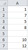
You’ll notice they’re not sorted and there is a blank cell in the middle of the range. So, our formula needs to be able to handle blanks and an unsorted list.
And here she is:
=SMALL(IF(COUNTIF($A$1:$A$7,ROW($1:$12))=0,ROW($1:$12),""),ROW(A1))
It’s an array formula so you need to enter it with CTRL+SHIFT+ENTER.
Below you can see the results of the formula copied down column C. When there are no more missing numbers it returns a #NUM! error.
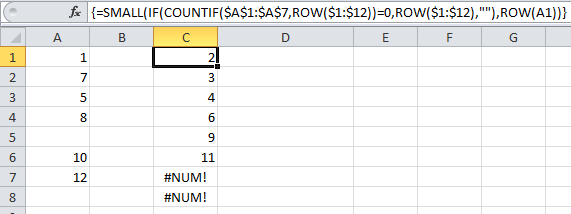
Tip: You can easily avoid the #NUM! errors by wrapping it in an IFERROR function if you prefer.
In English the Formula in Cell C1 Reads:
Count the numbers in the range A1:A7, that match the numbers generated by ROW($1:$12) i.e. {1;2;3;4;5;6;7;8;9;10;11;12}, if they = 0 (i.e. if they’re missing), give me a list of them, if they’re not = 0 (i.e. not missing), give me "" (i.e. nothing), and in this cell just return the 1st smallest missing value.
The cell reference in the ROW(A1) part of the formula is relative, so as you copy the formula down column C, ROW(A1) becomes ROW(A2) which =2 and returns the second smallest missing number, ROW(A3) which is 3, returns the third smallest missing number and so on.
Functions Used in this Formula
SMALL
The SMALL function returns the smallest kth value in an array. e.g the first smallest, second smallest, third smallest and so on.
The syntax is SMALL(array,k)
ROW
This ROW formula: ROW(A1) returns the row number of a reference. In this case it would return 1.
This ROW formula: ROW($1:$12) returns an array of values from 1 to 12 like this {1;2;3;4;5;6;7;8;9;10;11;12}. It works this way because this is an array formula entered with CTRL+SHIFT+ENTER.
COUNTIF
The COUNTIF function is counting the numbers in the range A1:A7 that match the array of values returned by the ROW function {1;2;3;4;5;6;7;8;9;10;11;12}.
The syntax is: COUNTIF(range, criteria)
IF
The IF function tests for counts of 0, and if TRUE i.e. zero (remember if the count is zero it means the number is missing), it then returns the corresponding value from the resultant array generated by ROW($1:$12) i.e. {1;2;3;4;5;6;7;8;9;10;11;12}, otherwise it returns nothing.
The syntax is: IF(logical_test, value_if_true, value_if_false)
Let’s Step Through How It Evaluates:
The key here is that array formulas evaluate on an array of items i.e. more than one item, within the one formula. Below you will see evidence of this as the formula evaluates.
=SMALL(IF(COUNTIF($A$1:$A$7,ROW($1:$12))=0,ROW($1:$12),""),ROW(A1))
Step 1 - The values in the range A1:A7 and ROW(1:12) are returned:
=SMALL(IF(COUNTIF({1;7;5;8;;10;12},{1;2;3;4;5;6;7;8;9;10;11;12})=0,ROW($1:$12),""),ROW(A1))
Step 2 - The COUNTIF then returns (a resultant array of) the counts of values in the array returned by the ROW(1:12) formula that are present in the range A1:A7:
=SMALL(IF({1;0;0;0;1;0;1;1;0;1;0;1})=0, ROW($1:$12),""),ROW(A1))
i.e. in the range A1:A7 there is 1 number 1 in the range, there are 0 number 2’s, 0 number 3’s etc.
Step 3 – The IF function’s logical test evaluates returning a TRUE where the number in the resultant array =0, and a FALSE where it doesn’t:
=SMALL(IF({FALSE;TRUE;TRUE;TRUE;FALSE;TRUE;FALSE;FALSE;TRUE;FALSE;TRUE;FALSE}, {1;2;3;4;5;6;7;8;9;10;11;12},""),ROW(A1))
Step 4 – the IF function’s value_if_true and value_if_false evaluate:
=SMALL({"";2;3;4; "";6;"";"";9; "";11;""},ROW(A1))
We now have a resultant array of the missing numbers.
Step 5 – The final ROW function evaluates to 1:
=SMALL({"";2;3;4; "";6;"";"";9; "";11;""},1)
Step 6 – the SMALL function finds the 1st smallest value in the array:
=2
Tip: the ROW function is used as a short cut to avoid having to type in an array constant. i.e. it’s quicker to type ROW($1:$12) than it is to type {1;2;3;4;5;6;7;8;9;10;11;12}
Note: This formula will ignore duplicate values in the list since it’s only looking for numbers in the range that have a count of 0, i.e. are missing.
Limitations of This Formula:
- It uses the ROW function to generate a list of values that should be in Deborah’s range. It is therefore limited to the number of rows in your workbook. If you’re using Excel 2003 you’re limited to numbers in the range 1 to 65,536, and if you’re using Excel 2007 onwards you’re limited to number between 1 and 1,048,576.
- It only works with positive numbers >0.
- It only works with whole numbers/integers.
Here is a clever VBA solution to find missing numbers that gets around some of the limitations above, plus the added bonus of allowing you to choose whether you want your list of missing values returned in a vertical or horizontal list.
Formula Challenge
What if your sequence of numbers were all negative. What formula would you use to find the missing negative numbers?
Please leave your answer in the comment field below.
Thanks
I’d like to thank Deborah for asking this question. It reminded me that I should write about this formula.
I’d also like to thank Oscar Cronquist of Get Digital Help for sharing his formula.


Hello,
I created the below formula based on the guidance provided in this article. For my needs, I don’t want it to pull any number that is missing, I want it to pull any number that is in a list in Sheet1 and not the current sheet. My formula works great, however I need it to be more flexible, in the scenario that additional numbers are added to the list in Sheet1, I don’t have to adjust the range in the formula each time. I tried adjusting the formula to reference only column D in Sheet1, but it returns zeros and blanks. Can you please advise on a solution?
=IFERROR(SMALL(IF(COUNTIF($F:$F,Sheet1!$D$3:$D$1868)=0,Sheet1D$3:$D$1868,””),ROW(A1)),””)
Thank you!
Hi Ally,
Can you please open a new topic on our forum, with a sample file attached, so we can see how your data looks like?
Basically, to make it flexible, Sheet1D$3:$D$1868 Should look like:
Sheet1!D$3:index(Sheet1!D:D,COUNTA(Sheet1!D:D))
Hey
im running a danish version of excel, but i changed , to ; and translated the commands and it works great
However my data starts in row 3 but the results ( missing numbers) starts i row 1
result is i dont get to see the first 2 numbers missing in the data…
how could i get this to start fraom row 3 ?
Hi,
Change $A$1:$A$7 with your range ($A$3:$A$700 for example). Also, change the 12 from ROW($1:$12) to your maximum number that can be found in that range.
Cheers,
Catalin
hi there, thanks for the insight you gave me,
actually i have a column with and index. index goes from 1 to 8.
so we have
name index
element 1 1
element 1 4
element 1 6
i can get for element 1 the elements as a set of data array 1 4 6 with something like if(C:C=E1;F:F;””) where it will check in E1 the name of the element and return the array of indexes. ive managed also to return with joinTEXT(….) this indexes for each element name.
but… for some reason it wont work if I put inside a COUNTIF … im not sure if excel is not liking the if (C:C=E1 part where I get an array resulting in all elements of my interest…
not sure if this is a limitation in excel …
15 minutes later i found the way. you cant use countif. need to use COUNTIFS and put 2 criteria. one is for returning all indexes found. it did work
thanks for the inspiration anyway
Glad you figured it out, Oswald.
I have spent hours looking up and reading everyones text and i am still hopelessly lost. if only someone could just show in a small display how to find 3, 4 or more numbers in a row of “consecutive cells” on an array or matrix of say 4 columns of cells contaning numbers I need to finish a ledger. I would be forever greatful. I try every possible formula configuration on the find and replace drop down dialog box without success. finding one number at a time. Is it possible to find multiple numbers at a time in consecutive cells? If you think you can help, thank you then for your valuable time and effort. John Hemmerling
Hi John, please post your question and sample Excel file with the example data and desired result on our forum and we’ll help you out. Mynda
Ok, let me try again. I am trying to find say numbers 345, 784, 3389 in one row, three consecutive cells. Is this even possible to do?
Hi John, please post your question in the forum with an Excel file containing some example data so I can see what you mean. There is always context that can’t be easily illustrated in a description that will dictate our answer. e.g. I can’t tell from this description how many columns of data in a row there is or whether it’s possible for this sequence of numbers to be present more than once in a row etc. An example will answer this and any other questions that may arise. Mynda
How do you apply this formula where you want to treat each row as a new set of range? Essentially want to compare Column 1 vs Column 2 row by row.
Column 1
Row 1 : 1000
Row 2 : 1014
Column 2
Row 1: 1002
Row 2: 1016
Hi,
So what is the purpose of your comparison? If I compare A1 to B1, then A2 to B2 etc, what am I checking for?
This type of question should be asked on our forum where you can supply your data. Please start a topic there.
Regards
Phil
Hello all please I need help.
I’m currently doing a research, I have numbers from 1 to 10731. Some numbers are missing in-between the 1 to 10731.
please how do I find the missing numbers using Excel?
HI,
Not sure what to say except have you tried using the information in this post?
If you’ve got a workbook where you’ve tried to get this to work but are having issues, then please post a topic on the forum and supply the workbook. That way we can see your data and be able to offer some help.
Regards
Phil
Hi, this is very helpful, but I am having trouble executing the code (using Excel 2016).
I have the following sequence of numbers:
8834
8835
8836
8837
8838
8839
8840
8841
8843
8845
8846
8847
8848
8851
8852
8853
8854
8855
8857
8858
8859
8860
First, I entered the code like this:
=SMALL(IF(COUNTIF($A$2:$A$23, ROW(8834:$8860))=0, ROW($8834:$8860),””), ROW(A1))
and it gave me just the first missing number
And it just gave me the first missing number (8842)
Then I tried this after reading some comments:
=SMALL(IF(COUNTIF($A$2:$A$23, ROW($2:$23))=0, ROW($2:$23),””), ROW(A1))
And this gave me 2..
Can you help me figure out where my mistake is?
Hi,
The first formula looks good in your case, have you copied down the formula? The results will never show in a single cell, you have to copy the formula down. Note that you should add a $ in the first range: ROW(8834:$8860), the reference to row 8834 is relative and will increase when copied down.
As original
sr. no. values
1 2.234
3 2.565
3 2.443
5 2.443
2 2.445
—————————————
excel filter use
sr. no. values
1 2.234
2 2.445
3 2.565
3 2.443
5 2.443
——————————————-
Q.How to and i want to?
sr. no. values
1 2.234
2 2.445
3 2.565
3 2.443
4 missing
5 2.443
**create automatic “4” sr. no. and other nos.
——————————————-
Hi Sujit,
This post is about finding missing numbers in a sequence, but your numbers are not in a sequence.
I don’t see any pattern to your numbers so I’m not sure how you want to guess the missing value, or the ‘other numbers’ ? You could use an interpolation algorithm to estimate missing values, but in the example here, there is only 1 missing and my interpolation calculates it at 2.443.
You’ll need to provide more data points in order to get a more useful result.
Regards
Phil
Thank you so much for this, ma’am!
You’re welcome
What if the lists are in rows instead of column?
Hi Adamu,
The formula will work exactly the same with no change, no matter if the list is horizontal or vertical:
=SMALL(IF(COUNTIF(A$1:F$1,ROW($1:$12))=0,ROW($1:$12),””),ROW(A1)) and
=SMALL(IF(COUNTIF($A$1:$A$7,ROW($1:$12))=0,ROW($1:$12),””),ROW(B1))
will give the same result if, of course, you have the same numbers in those ranges.
Hope you already tried that.
Cheers,
Catalin
WHAT IF THE RANGE OF NUMBERS IS A COUPLE 1000 NUMBERS?
It will work fine with 2000+ numbers.
If you are having some issues please create a topic on the forum with an example workbook.
Regards
Phil
OGP NOS INVOICE#
=SMALL(IF(COUNTIF($A$2:$A$361,ROW($2:$361))=0,ROW($2:$361),””),ROW(A1))
54685 32119 2
54686 32120 #NUM!
54688 32121 #NUM!
54689 32122 #NUM!
54690 32123 #NUM!
54691 32124 #NUM!
54692 32125 #NUM!
54693 32126 #NUM!
54694 32127 #NUM!
54695 32128 #NUM!
54696 32129 #NUM!
54699 32130 #NUM!
54700 32131 #NUM!
54701 32132 #NUM!
54702 32133 #NUM!
54703 32134 #NUM!
54704 32135 #NUM!
54705 32136 #NUM!
54706 32137 #NUM!
54707 32138 #NUM!
54708 32139 #NUM!
54709 32140 #NUM!
54710 32141 #NUM!
54711 32142 #NUM!
54712 32143 #NUM!
54713 32144 #NUM!
Hi Muhammad,
Please upload a sample file on our forum (create a new topic after sign-in)
Just a list of values is not enough to understand what you did there.
See you on forum.
Catalin
need help please
Please post your question on our Excel support forum.
I am working with invoice numbers entered manually into a large worksheet that is vital to tracking cost and sales margins. Each invoice number may have multiple line items if there is more than 1 item on the invoice. Sometimes during the course of the year I fail to input an invoice number because of the multiple places I have to put that information and the sheer volume of invoices on some days and don’t realize it until the invoice is paid. The list is in a table format so the range is named. The list grows daily. Each year I would have a new starting invoice number.
My invoice numbers are in column O entitled Inv#. I need it to either highlight the two numbers around which the invoice number is missing or list it on a separate sheet in the workbook.
Hi Trish,
Can you upload a sample file on our forum so we can see your data structure? (create a new topic after sign-up)
Thank you
Catalin
I am a working Librarian and was presently in the processing of carrying out stock verification of books, around 40 thousand numerical accession numbers. I was in search of this type of formula. Thanks a lot for your people for sharing your wit and expertise. I am really thankful and hope you will be sharing your knowledge with same spirit in future, as well, simply for the betterment of the humanity.
You’re welcome, glad you found this useful.
Phil
I am currently trying to find away to find missing numbers in a sequence, but want the formula to reference a number in a cell to change the range. For example, In cell A1 I have the formula =sum($b$1:$b$8)
I want to replace ONLY THE 8 above with a cell reference…for example in cell D1 I have the number 9. So I’m trying to use that same formula logic =SUM(INDIRECT(“B1:B”&D1)) in the missing sequence formula so that I don’t have to update the formula each time I paste in new data.
In the Formula below the number for the start of the range is in H2 the end of the range in J2 and the range of numbers is in column I and the start of the missing list start is J4.
It with either tell me too many arguments or formula is broken. Please help if you can fix.
=SMALL(IF(COUNTIF(I$4:I$1048576,ROW(INDIRECT(“I”&H2):INDIRECT(“I”&J2))=0,ROW(INDIRECT(“I”&H2):INDIRECT(“I”&J2),””),ROW(J4))
Hi Bryan,
No idea what your formula does, looks really messy.
Just to correct the functional errors:
=SMALL(IF(COUNTIF(I$4:I$1048576,ROW(INDIRECT("I"&H2):INDIRECT("I"&J2)))=0,ROW(INDIRECT("I"&H2):INDIRECT("I"&J2)),""),ROW(J4))Great job!
Thank you, Mynda!
For myself, I’d use a helper column to convert the negatives to positive numbers, run the array formula, and then convert the output back to a negative number.
Using the same idea of a helper column, non-integers can be assessed. Multiply the original value by powers of 10 until you get an integer and process it. Convert the output back by dividing by the same power of 10 as used previously. A few extra steps are needed to finish the process. First, use a round function to get the right number of decimal places. Copy and paste the values into the list you’re trying to generate. Lastly, highlight the values you just pasted and remove the duplicates. A bit complicated, but it works.
Cheers, Ruthie. I like your solution for handling non-integers too 🙂
hi Mynda!
the second Limitation can be solve:
then we can write a general solution so:
where rng is $A$1:$A$7
regards
r
Ciao r,
Your ‘general solution’ is ideal in that it handles negative right through to positive, including zero. And perhaps best of all it detects the size of the number range. Brilliant!
Thanks for sharing.
Mynda.