Excel Multi-cell Array Formulas

Excel Multi-cell array formulas are a single formula which returns multiple values and is entered into multiple cells. Hence ‘multi’ in the name.

Let’s look at an example, say we want to return a list of numbers 1 through 10 in cells A1:A10.

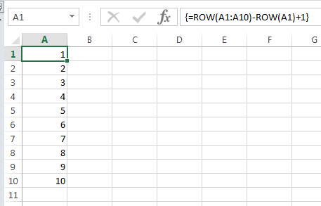
Step 1 – very important; first select cells A1 to A10

Step 2 – type in this formula; =ROW(1:10)

It should look like the image below with the formula in cell A1:

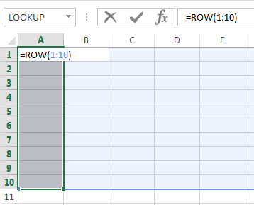
Tip: ROW(A1:A10) or ROW($A$1:$A$10) yields the same results as ROW(1:10).

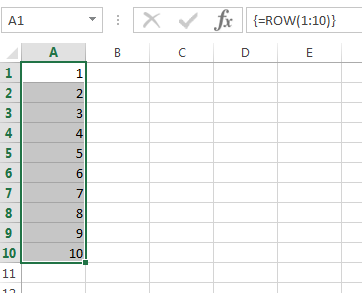
Step 3 – press CTRL+SHIFT+ENTER to complete the formula.

You should have the numbers 1 through 10 in cells A1:A10 and in the formula bar you’ll see the curly braces around your formula as shown below:

Features of Excel Multi-cell Array Formulas

1. If you select any of the cells in the range A1:A10 you’ll see the formula is exactly the same. In effect the range 1:10 is absolute yet I haven’t had to use the $ sign to lock them in.
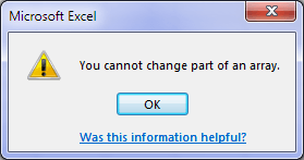
2. If you try to delete or insert cells or rows between A1:A10 you’ll get this error:
3. To select all of the cells relating to the array formula select one cell containing the formula and press CTRL+/
   

   

4. To edit the formula simply click on any of the cells in the array, make your changes and press CTRL+SHIFT+ENTER to re-enter the formula.
5. To delete a multi-cell array formula first select the array, in this case cells A1:A10 (remember the keyboard shortcut is CTRL+/), then press DELETE. Alternatively you can delete all of the rows or the column containing the formula.

Multi-cell Array Formula Gotchas

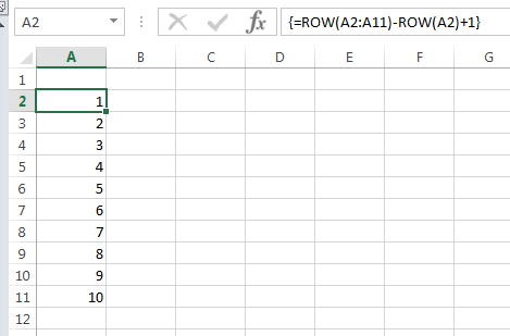
While you can’t insert rows or cells within an array, you can insert rows above and this may alter the results of your formula. For example, if I insert a row above cell A1 my formulas and cell references adjust like so:

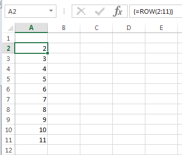
This can be catastrophic for your formula, especially if you’re nesting ROW in another formula and the impact is not transparent like the example above.

The solution is to use this formula instead of ROW(1:10):

=ROW(A1:A10)-ROW(A1)+1

Now when I insert a row above A1 my formula adjusts but I still get numbers 1 through 10:

Tip: you can insert numbers 1 through 10 across a row with this multi-cell array formula:

=COLUMN(A1:J1)-COLUMN(A1)+1

Don’t forget to press CTRL+SHIFT+ENTER to complete the formula.

When to use Multi-cell Array Formulas

We could just as easily insert the numbers 1 through 10 in column A with this formula (entered in any cell):

=ROW(A1)

Then copy down as needed. Of course this formula is subject to error if rows are inserted above it, so you’re better off using the ROWS function like this:

=ROWS($A$1:A1) or =ROWS($1:1)

And don’t forget there’s always Auto-fill or Fill Series for a quick list of numbers.

However, the benefit of using a multi-cell array formula is that it prevents rows/cells being inserted within the range without the need for worksheet protection.

Multi-cell Array Formula Examples

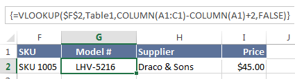
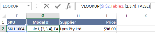
So far we’ve looked at a basic example, but often you’ll find more complex multi-cell array formulas that contain nested functions like this VLOOKUP with COLUMN in cells G2:I2:

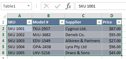
I’ll explain; I have an Excel Table in cells A1:D6 called Table1:

And in cell F2 I have a data validation list containing the SKU’s:

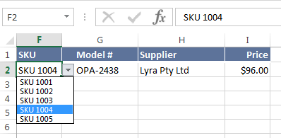
When I choose an SKU from the Data Validation list a multi-cell VLOOKUP array formula in cells G2:I2 returns the Model#, Supplier and Price for the selected SKU:

The only difference between this multi-cell VLOOKUP array formula and a regular VLOOKUP formula is the COLUMN functions used to return the col_index_num argument for VLOOKUP.

When evaluated COLUMN returns an array {2,3,4} for the col_index_num, as you can see below:

And because I’ve selected 3 cells for my multi-cell array formula it returns the value from 2^nd column in Table1 to cell G2, the value from the 3^rd column in H2 and the value from the 4^th column in I2.

Remember the main benefit of this formula over a regular VLOOKUP is that you can’t insert columns between G and I.

The other benefit is that if an inexperienced user attempts to edit this formula they’re likely to get the error message “you cannot change part of an array”, and that might just be enough to prevent them from messing up your formulas. No promises though. Those users can be tenacious 😉

Multi-cell Array Formula Functions

There are also quite a few functions in Excel that return an array of results. That is they return multiple values and deposit each one in its own cell.

For example the FREQUENCY function does this. The syntax is:

FREQUENCY(data_array, bins_array)

FREQUENCY calculates how often values occur within a range (data_array), for each value in the bins_array. Let’s look at an example:

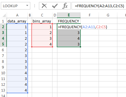
Column A contains a series of values (our data_array). We want to count how often each number in column A occurs. In column C we have our bins_array, which is simply a list of distinct numbers from column A.

In column E we enter our FREQUENCY formula by first selecting 4 cells (E2:E5, one for each bin), then the formula:

=FREQUENCY(A2:A13,C2:C5)

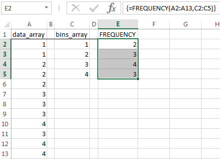
Press CTRL+SHIFT+ENTER to complete the formula.

The image below shows the FREQUENCY formula has counted 2 occurrences of the number 1 in our data_array, 3 occurrences of number 2 and so on:

Advantages of multi-cell array formulas

• User error more easily avoided since editing them is difficult unless you know how.
• Prevents inserting rows/columns within the array range, but not above or below.

Caution

Array formulas applied to large data sets can be slow and inefficient so use them with caution.

Thanks

Thanks to Mike Girvin and his incredible book CTRL+SHIFT+ENTER Mastering Excel Array Formulas. I learnt endless tips in this book. It’s a must read for any Excel enthusiast.

Thanks to Simlaoui’s comment on last week’s post on the ROW function which inspired me to write about multi-cell array formulas.

Disclosure: if you purchase Mike's book I earn a couple of dollars. That's not why I recommend it though. It's a brilliant book and you'll learn a lot, even if you're already familiar with array formulas.