Last week I had an email from Mike asking how he can lookup a suburb in a range of columns and return the post code from the header row.
I imagine his data was a bit like this:
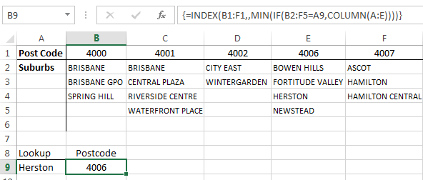
And in cell B9 he wants to find the post code for Herston.
One way is with this array formula:
=INDEX(B1:F1,,MIN(IF(B2:F5=A9,COLUMN(A:E))))
Entered with CTRL+SHIFT+ENTER.
Enter your email address below to download the sample workbook.
Before we dive in, here are the syntaxes for the INDEX and IF functions as a reminder (I’ve crossed out the arguments we’re not using):
INDEX(reference,row_num,[column_num],[area_num])
IF(logical_test, [value_if_true],[value_if_false])
The INDEX formula is returning a reference to the cell in the first row for the column containing ‘Herston’. For the column_num argument it uses a combination of IF, COLUMN and MIN.
Here it is again for reference:
=INDEX(B1:F1,,MIN(IF(B2:F5=A9,COLUMN(A:E))))
In English the above formula reads:
Check the cells in the range B2:F5 for 'Herston' and tell INDEX what column number it's in. i.e. column 4. INDEX (look in) the range B1:F1 and return a reference to the 4th cell i.e. E1, which contains 4006.
So what’s MIN got to do with it….hold your horses, more on that in a moment.
Let’s step through the formula in the order it evaluates:
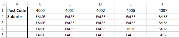
Step 1 - IF function’s logical_test: B2:F5=A9 i.e. B2:F5=Herston and it looks like this:
=INDEX(B1:F1,,MIN(IF({FALSE,FALSE,FALSE,FALSE,FALSE; FALSE,FALSE,FALSE,FALSE,FALSE; FALSE,FALSE,FALSE,TRUE,FALSE; FALSE,FALSE,FALSE,FALSE,FALSE},,COLUMN(A:E))))
Tip: did you notice in the formula above there is a semicolon after every 5th ‘FALSE’ instead of a comma. This semicolon represents a new row in the array.
Or if you imagine our formula is putting together a list of values representing each row in the table like this:
Step 2 - COLUMN function: This evaluates to return a horizontal array of numbers {1,2,3,4,5} for our IF function’s value_if_true argument. These numbers represent the 5 columns B:F in our table.
Our formula now looks like this:
=INDEX(B1:F1,,MIN(IF({FALSE,FALSE,FALSE,FALSE,FALSE; FALSE,FALSE,FALSE,FALSE,FALSE; FALSE,FALSE,FALSE,TRUE,FALSE; FALSE,FALSE,FALSE,FALSE,FALSE}, {1,2,3,4,5})))
Tip: Instead of using the COLUMN function to generate the array of numbers we could simply type {1,2,3,4,5} into the formula. However, with large horizontal arrays it’s quicker (and dynamic) if we use the COLUMN function to generate the array, or for vertical arrays you can use the ROW function.
Note: if you don’t want your COLUMN function to be dynamic you can use the INDIRECT function to fix it, like this:
=INDEX(B1:F1,,MIN(IF(B2:F5=A9,COLUMN(INDIRECT("A:E")))))
Step 3 - IF function value_if_true: The IF function finishes evaluating by assigning the value_if_true numbers (generated by the COLUMN function) to the TRUE results in the logical_test.
To visualise this we can look at the 3rd horizontal array (i.e. the series of FALSE/TRUE after the second semicolon below). Remember this is the 3rd row of our table above.
Excel gives the TRUE results the corresponding number from the array generated from the COLUMN function {1,2,3,4,5} like so:
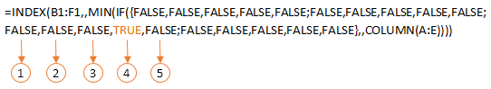
Note: In this step the FALSE values evaluate to nothing i.e. they are ignored. Remember we don’t have a value_if_false argument in our IF formula. Our formula now looks like this:

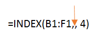
Step 4 – MIN: This simply evaluates to find the one and only number; 4.
=INDEX(B1:F1,, 4)
Tip: Since there is only one number remaining (the rest are all FALSE) we could have used MAX or SUM to get the same result as MIN.
Step 5 – INDEX: Finally INDEX can return a reference to the 4th column in the range B1:F1 which is cell E1 containing post code 4006.
Tip: Notice how our INDEX formula doesn’t have a row_num argument:
Since our reference is only one row high we don’t have to type a 1 in for the row_num argument, we simply enter a comma as a placeholder and continue on to the column_num argument.
What The?
Did you find that tricky?
When working with long or complex formulas I like to use the Evaluate Formula tool to understand what’s going on behind the scenes.
You can also evaluate parts of your formula by highlighting the section of the function in the formula bar and pressing the F9 key. Below I’ve evaluated the COLUMN(A:E) part of my formula:

To revert to the original formula either press the escape key or CTRL+Z.

Hi Mynda this was really helpful, I am dealing with a similar scenario but i want to do a two way match. For example column A had different cities listed and different cities could have the same suburb names, so how will we modify the formula in that case? thanks
Hi Muhammad,
Not sure what you want the desired result to be. Please post your question on our Excel forum where you can also upload a sample file and we can help you further
Mynda
Hello, I know this is a really old post but I’m running into trouble that I’m hoping someone could help me with. In the screenshot (linked below) I’m trying to have reach row in column BB to return the column header of the cell that is populated between columns O:U. There will never be values in multiple columns in the same row.
I’m getting a #REF error for some reason, and you can see my formula.. what did I do wrong?
https://prnt.sc/FtSrIJbPrMYg
Hi Daniel,
Try this formula:
As explained here: Find the first or last value in a range.
MFind the first or last value in a range
Thanks Mynda, but that just seem to give me the value of the cell 1up + 1over.. see screenshot:
https://prnt.sc/LmorRJ0gpoId
I also am looking for it to return the title of the column that contains the value, or at least the column number
Looks like you didn’t set the cell references to absolute. i.e.
Mynda
thanks, but for some reason that doesn’t seem to do the trick. row 2 is working but all the other are incorrectly returning “Geo:Zip Code”.
https://prnt.sc/M6ZG9Z48QpsU
I can’t tell anything from the screenshot because I can’t see the formula bar. Please post your question on our Excel forum where you can also upload a sample file and we can help you further.
This is exactly what I needed. Thank you!
Glad we could help 🙂
This is very cool. How would you modify the formulas if an item appeared in more than one column and you want to see ALL matched columns?
If you have Microsoft 365 you can use the new array functions:
=FILTER(HSTACK(TOCOL(CHOOSEROWS(B1:F1,{1,1,1,1})),TOCOL(CHOOSEROWS(B1:F5,{2,3,4,5}))),TOCOL(CHOOSEROWS(B1:F5,{2,3,4,5})="Herston"))Mynda
Great idea! However, Brisbane in shown under two postal codes (4000 and 4001), yet only the first one is shown in the search. How could this formula be modified to show all matches.
You could use the FILTER function:
=FILTER(B1:F1,B2:F2=”Brisbane”)
or for vertical results:
=TRANSPOSE(FILTER(B1:F1,B2:F2=”Brisbane”))
Hello,
I am attempting to use your formula in a similar application. The only difference is I want to use two columns that have the same heading (i.e. if I had two columns with a 4000 postal code, to use your example) and I am having trouble with generating the column index for each column. In your example, you used the MIN function, but there was only one value. Any suggestions?
Thank you,
Hi Marco,
I’m not sure there’s a solution to this other than not having multiple columns with the same heading. It doesn’t make sense to me why you would have two columns that are the same. Why not put the data into one column. If they’re not the same, then give the columns different names.
Mynda
superb explanations and clever tools – thank you
Glad it was helpful, Grant!
Hi, Nice solution. But I’m having an error in the conditional IF. I don’t know why the range (B2:F5=A9) is causing problems. I had test every variable and I’m 100% sure that is the range. What can I do?
Here is my formula:
INDEX(C2:Y2,,MIN(IF(IFERROR(C24:Y24=AB24,0),COLUMN(A:Y))))
Thanks!
Hi Billy,
I think it’s best that you post your question and sample Excel file here on our forum, so we can see your formula in context of your file because there are a few things preventing it evaluating. e.g. COLUMN(A:Y) returns more values than the INDEX array (it should be COLUMN(A:W)), so this will throw the error every time. IFERROR is redundant. If no cells in C24:Y24 = AB24, INDEX will return the whole array, but if you don’t have dynamic arrays you will only see the first value.
Mynda
Hi there!
I know this is quite an old thread but I recently came upon it for a project I’m working on. It’s very similar to the example problem except reversed. I want to be able to input a postal code and have my excel array output the associated city. The array is organized in columns with each header being a city and the postal codes listed vertically beneath them. This function is working quite well except I notice that if I input a postal code that is not contained in the array, the function automatically outputs the column header of the first column rather than 0 or NA or something like that. Can you recommend a way of fixing that so it’s clear that the function could not find the postal code in the array?
Thank you very much!
Hi Jack,
When you supply INDEX with a reference (in this case the column number) of 0, it returns all the columns. When you are trying to look up a postal code that is not in the lookup array, the formula is effectively passing 0 into INDEX so it returns all your column headers. But because you’ve got it entered as an array formula, you’re only seeing the first column header.
You can fix this by using this
The first IF/MIN is modified to return -1 if your postal code is not found. The -1 will cause an error in INDEX so the IFERROR catches that and returns a null string “”
There is a caveat with this. If your lookup array contains empty cells, then when you don’t specify an input to the formula, from cell A9 in this case (taken from the example workbook), you’ll get the column header returned where the first empty cell occurs.
So either don’t have empty cells in your lookup array or always specify something to lookup e.g. a hyphen, rather than leave the cell containing what you want to lookup empty.
Cheers
Phil
This formula is very useful, thanks! I am having a problem though, My table doesnt begin in column A or B but rather in column Z and I can only get it to work if my table begins in column A or B but I have other data in those columns. I’ve tried selecting different ranges for the COLUMN, but it just doesnt work. Can you help me with this?
Thanks!
Hi Oscar,
I suspect you changed the COLUMN part of the formula to match your data starting column, but that’s not the purpose of COLUMN. Please read “Step 2 – COLUMN function” again and see if that’s your problem.
Mynda
Very helpful. Do you think it’s possible to use the same concept to find the first column with a value in a range dinamically?
Hi Gabriela,
Do you mean like this: https://www.myonlinetraininghub.com/return-the-first-and-last-values-in-a-range
Mynda
I have the following table as a sample: A B C D E F G 1 Copper90 Copper75 Copper90 85 2 100 95 110 105 3 90 87 100 97 4 80 78 90 88 I hope to have a formula in G1 that will take the value in E1 and look for which column contains that value in row 1 range (A1:B1). Then, I thought the match function with match type -1 look for the smallest value in that column (?2:?4) that is = or > than value in F1. Finally, I would like to offset the matching cell by 2 columns to the right and copy and paste this value. In this example G1 = 100. If E1 was Copper75, G1 would be 97. I have tried several formulas with index, lookup, match functions, but have been unsuccessful. I can reconfigure the table if it makes the result I am looking for possible. Any advice would be greatly appreciated.
Hi Marshall,
Can you please send me your file via the help desk as the formatting of your data didn’t come through very well in your comment.
Thanks,
Mynda.
Its Simply Superb…!!! I’m in love with your website…!!<3
Cheers…!!:)
Aw, thanks Krishna 🙂 Glad you love it.
Mynda, I’m struggling with what should be the simplest part of this formula – COLUMN. Why is it that when I break out that part of the formula and just type {=COLUMN(A:E)}, it returns a value of 1 rather than 1,2,3,4,5?
Hi Michael,
When you enter =COLUMN(A:E) in a single cell it can only return the first result, which is 1.
If you were to first higlight 5 cells (across a row) and then type in =COLUMN(A:E) and enter it as an array formula with CSE you will get a 1 in the first cell, a 2 in the second cell, a 3 in the third cell and so on.
This is a multi-cell array.
I hope that helps.
Kind regards,
Mynda.
Thanks, Mynda. Little by little I’m getting it through my thick skull!
You’re welcome 🙂
Very clever formula 🙂
Thanks!
Thank you, Piotr 🙂
I’m in love with SUMPRODUCT recently and I rebuild your cool formula so it doesn’t require CSE 🙂
=INDEX(B1:F1,,SUMPRODUCT((B2:F5=A9)*COLUMN(A:E)))
Love it, Piotr. Thanks for sharing 🙂
This is Amaaaaazzzzzzing…. U r a Star Mynda…
I really love the way you explained it…. thanks
Wow, thank you, Pradeep 🙂